Object Orientation: Observer Pattern

The observer pattern is a simple yet quintessential design pattern in object oriented programming. As programs become larger, objects multiply quickly, as do the interactions between them. For example, a class instance can be contained as an attribute in another class (composition), or be used by some method in another class (association). Sometimes these class relations are very simple and can be used without a second thought. But let’s assume you have some class containing mutable information (the “subject” class) that is potentially relevant to a larger amount of other classes that observe the subject class. Rather than constantly spamming the subject class to ask whether its information has changed, a lazy and efficient method is preferred: let the subject class keep track of all classes requiring its information and notify them that a change has been made.

Let’s further assume that although we currently have some classes using this information, there could be more or less other observing classes in the future that we want to add. We could of course directly have the subject class contain instances on all observing classes and call methods on all these observers–a direct coupling between the subject and all its observers–but this makes the subject class more complicated than necessary and harder to maintain, as it needs to know about many different objects. This is where the observer pattern comes in. Rather than using this direct coupling to code the one-to-many dependency, we only require the subject class to inform its observers when a change to it is made, without having to specify what to do based on this change. The latter is best delegated to all the different observing classes themselves. Let’s write up a quick and light-hearted example.

As I write this, the Nijmeegse Vierdaagse (the biggest walking event in the world) is going on, and alcohol flows freely through the streets. But of course, not everyone has a healthy relationship with alcohol. After drinking for seven days straight, a not to be specified person realizes he or she might have a problem and decides to see a therapist who starts to observe this person’s behavior.

First, we define the alcoholic:

import java.util.Observable;
import java.util.Observer;

public class Alcoholic extends Observable {
    private int beersDrank;
    private String name;
    
    public Alcoholic(String name, Observer therapist){
        beersDrank=0;
        this.name=name;
        addObserver(therapist);
    }
    
    public void drinkBeer(){
        beersDrank++;
        setChanged();
        notifyObservers();
    }
    
    public int getBeersDrank(){
        return beersDrank;
    }
    
    public String getName(){
        return name;
    }
}

We are speaking here of the cheap kind of alcoholic that only drinks beers. An alcoholic has some name that the therapist can ask for with a getter. Moreover, we keep track of how much beers the alcoholic drank. The Observer pattern is natively implemented in Java, so to use it we import the Observable class and extend it. Within the Observer pattern, this alcoholic is defined as the observable “subject” class. As said before, it only needs to keep track of its observers so it can notify when a relevant change has been made. In this case, we add a Therapist as an observer with addObserver(new Therapist()). A change to the internals of the alcoholic is made every time a beer is drank (poor liver), so that is the situation in which we notify the observers with notifyObservers(). Now we only need to define the observing Therapist:

import java.util.Observer;

public class Therapist implements Observer {

    int beersObserved;
    
    public Therapist(){
        beersObserved=0;
    }
    
    @Override
    public void update(Observable o, Object arg) {
        if (o.getClass()==Alcoholic.class && o !=null){
            Alcoholic aa = (Alcoholic) o;
            beersObserved++;
            System.out.println("Therapist says: " + aa.getName() + " you already had " + aa.getBeersDrank() + " beers. That's enough!");
        }
    }

    public int getBeersObserved(){
 return beersObserved;
    }
}

The therapist can observe multiple alcoholics in parallel and keeps track of the total amount of beers it has observed. Whenever an observed alcoholic drinks a beer and notifies its observer (the therapist in this case), the therapist knows it has to update its knowledge of the observed class. The Observer interface provides the update function that is called whenever the alcoholic calls the notifyObservers() function. It is possible that the therapist also observes other kinds of patients that are not alcoholics, so we need to distinguish what the therapist does for what kind of patient. In our case, we only care about alcoholics, but to be complete we still check the class of the object we observe to take the appropriate action. In this case we simply give the alcoholic a small preach every time he or she has a beer (probably not so effective, but hey I’m not a therapist myself).

Let’s test our code:

    public static void main(String[] args) {
        Therapist therapist = new Therapist();
        Alcoholic student1 = new Alcoholic("Student1",therapist);
        Alcoholic student2 = new Alcoholic("Student2",therapist);
        
        student1.drinkBeer();
        student2.drinkBeer();
        student1.drinkBeer();
        student1.drinkBeer();
        student2.drinkBeer();
        
        System.out.println("The therapist counted " + therapist.getBeersObserved()+" beers.");
    }

Which gives the output:

Therapist says: Student1 you already had 1 beers. That's enough!
Therapist says: Student2 you already had 1 beers. That's enough!
Therapist says: Student1 you already had 2 beers. That's enough!
Therapist says: Student1 you already had 3 beers. That's enough!
Therapist says: Student2 you already had 2 beers. That's enough!
The therapist counted 5 beers.

Although the Observer pattern is in essence simple, its importance cannot be overstated. It is for example very important in the MVC-architecture that advocates a separation between model, view, and controller. The controller can make adjustments to the model, containing the program logic, and various “view” classes designed to display the model need to be informed about updates in the model effectively without becoming entangled with the model. The observer pattern takes care of just that.

Object Orientation: Strategy Pattern

In object-oriented programming classes tend to multiply quickly. Luckily, some design patterns are available to solve commonly occurring issues. In this post I want to quickly illustrate the strategy pattern with an easy example written in Java. To make it intuitively clear why this pattern is called the ‘strategy’ pattern, let’s sketch a situation in which the application of different strategies is important: a game.

Without getting lost in the philosophical details of what constitutes a game, we can safely assume a game at least needs players. So let’s make a Player class. We want a player to have a name, a team, and a game strategy:

public class Player {

    private String name;
    private Team team;
    private Strategy strategy;

    public Player(String name, Team team, Strategy strategy){
        this.name=name;
        this.team=team;
        this.strategy=strategy;
    }

    public String yell(){
        return this.name+" yells: "+team.yell();
    }

    public void changeTeam(){
        this.team=team.other();
    }

    public String getName(){
        return this.name;
    }

    public Team getTeam(){
        return this.team;
    }

    public String getStrategy() {
        return this.name+"'s strategy: "+this.strategy.sayStrategy();
    }

    public void setStrategy(Strategy strategy) {
        this.strategy=strategy;
    }
}

This class definition requires us to define at least two other classes, one for defining what a team is and another for determining the player strategy. Let us assume that for this particular imaginary game (we haven’t defined any actual rules), there are only two teams per game: a blue and a red team. Since blue and red are the only possible team instances, we can use an enumeration type. For some reason each team has an incredibly silly yell:

public enum Team {
    RED,BLUE;
    public String yell(){
        switch (this) {
            case RED: return "We are the red devils!";
            case BLUE: return "Blue is the color of righteousness!";
            default: return "";
        }
    }
}

Now the strategy pattern comes into play. We want each player to potentially have a different game strategy. A naive solution would be to create different player classes. We could have one class called CheatingPlayer and one class called FairPlayer and so on for all potential strategies. However, each of these classes will have the exact same code except for the code defining the strategy. Unnecessary code duplication must always be avoided. If you for example want to change some characteristic of the player, you would have to edit all duplicate code in all these classes. The strategy pattern solves this issue.

As we saw, we have a single Player class that has a Strategy as an attribute, but other than this we do not specify yet what particular strategy. The player could have whatever strategy, the only obligation we make now is that it has one. The solution is to make Strategy an interface defining what obligations each particular strategy should fulfill. Normally a strategy should have some influence on the player’s behavior in the game, but since we don’t program the game itself to keep it simple, we just want players to state their strategy when asked:

public interface Strategy {
    public String sayStrategy();
}

Each particular strategy has to define which String this function returns. For simplicity, let’s assume for now there are two particular strategies implementing the Strategy interface, one where we intend to cheat, and one where we will play fairly (whatever that means):

public class CheatingStrategy implements Strategy {

    @Override
    public String sayStrategy() {
        return "Sedating the enemy team with horse tranquilizer";
    }
}

public class FairStrategy implements Strategy {

    @Override
    public String sayStrategy() {
        return "Shaking hands, wishing the opponent good luck (because they need it)";
    }

}

We can create as many strategies as we see fit, and our problem is solved: each player can have a different strategy without having to define multiple player classes with duplicate code. Let’s see how it works:

public class StrategyPattern {
    public static void main(String[] args) {

        Strategy cheating = new CheatingStrategy();
        Strategy fair = new FairStrategy();
        Player Edwin = new Player("Edwin",Team.BLUE,fair);
        Player Diablo = new Player("Diablo",Team.RED,cheating);
        System.out.println(Edwin.yell());
        System.out.println(Diablo.yell());
        System.out.println(Edwin.getStrategy());
        System.out.println(Diablo.getStrategy());
    }
}

The console output is:

Edwin yells: Blue is the color of righteousness!
Diablo yells: We are the red devils!
Edwin’s strategy: Shaking hands, wishing the opponent good luck (because they need it)
Diablo’s strategy: Sedating the enemy team with horse tranquilizer

Calculating pi with Monte Carlo simulation

I came across Monte Carlo sampling in a class on Bayesian statistics, where a Markov Chain Monte Carlo (MCMC) sampler was used to approximate probability distributions that were otherwise hard to calculate due to nasty integrals. This posts illustrates the basic idea of Monte Carlo sampling, by using it to approximate the number $\pi$.

The basic procedure is as follows:

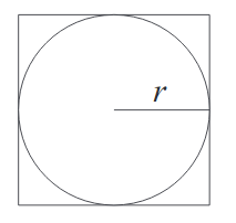
• Take a circle with radius $r$
• The area of the circle is $\pi r^2$
• Draw a containing square which then has area $(2r)^2=4r^2$.
• Sample points randomly within the square, and count how many fall within the circle
• Calculate the proportion of samples within the circle to the total amount of samples, and multiply by 4 to approximate $\pi$.

How does it work? ¶

Now we ask: what is the probability that any randomly sampled point within the square lands in the circle? This probability is the proportion of the area of the circle with respect to the total area (i.e. that of the square). We don’t want the sampling itself to influence the results, so having a uniform distribution to sample from is important.

Thus the probability that a randomly generated point lands in the circle is: $$\frac{\pi r^2}{4r^2} = \frac{\pi}{4}$$

This means that if we accurately approach the probability of a random point landing in the circle, we end up with a fourth of $\pi$. The law of large numbers states that if we repeat this experiment often enough the average of the results approaches the expected value, which is a fourth of $\pi$ in this case. It is no wonder that this method is called Monte Carlo: you might win a few games, but on average the casino always wins in the long run.

We can generate points with x and y coordinates uniformly sampled between -1 and 1. This effectively amounts to saying that for the circle we use a radius of 1, centered in (0,0). Now we need to determine a test for whether any given point lies in the circle. Given a sampled point, we can reconstruct if it lies on a circle with a radius smaller than 1. The radius is obtained with the “hypot” function, i.e. $\sqrt{x^2+y^2}$. If the reconstructed radius is smaller than the radius of our circle, we know it must lie within the circle we defined with radius 1. Otherwise, we know it is a point that only lies within the containing square, but not in the circle.

To get the probability we are interested in, we only have to divide the number of sampled points within the square by the total amount of samples. To get an approximation of $\pi$, we multiply this probability with 4.

Python script ¶

This is the python 3 script I wrote, so you can play around with the parameters yourself. The code for a simple histogram plot is also included, but you should delete this if you don’t have the matplotlib package (and don’t want to install it).

import random
import math
import matplotlib.pyplot as plt

radius=1
samples=10**6
iterations=100
countdown=iterations+1
estimations=[]

for i in range(iterations):
    sample_inside=0
    for sample in range(1,samples+1):
        hyp_r = math.hypot(random.uniform(-radius,radius),random.uniform(-radius,radius))
        if hyp_r < radius: sample_inside +=1
    countdown-=1
    print(countdown)
    estimations.append(4.0 * sample_inside / sample)
print("Approximation of pi: ", sum(estimations)/float(iterations))

bins=int(iterations/2)
plt.hist(estimations, bins=bins,histtype='step')
plt.savefig("pi-plot.png")

Sampling and Plots ¶

Another question is how much samples we need: a lot. Without working out the mathematics, some quick and dirty testing shows that in order to get only one decimal accuracy we already need at least 10.000 samples. Unfortunately, to get more accuracy, we need relatively more and more samples, since the rate of convergence is the inverse of the square root of the number of samples N. In simple words: the higher the number of samples we take, the slower the convergence.

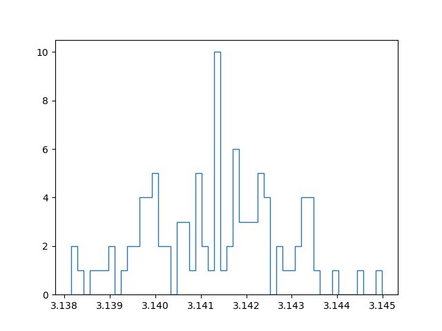
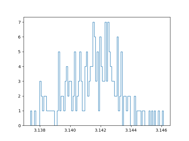
With a million samples, we can approximate the first two decimals well, but for the third decimals we already start getting into trouble. On top of that, the approximation becomes slow… Instead of straightforwardly pumping up the number of samples taken to increase the accuracy, I tried out another strategy. Instead of running a simulation with for example 100 million samples, I tried running 100 simulations with a million samples, and taking the average of those for the final approximation. In this manner we can create a confidence interval and say something about how reliable our estimate is. Since all samples are independent and concern a stochastic variable, the central limit theorem applies. In other words: if we have enough approximations, these approximations themselves will follow a normal distribution. I have an ongoing discussion with some friends about the benefit of this method, compared to running one bigger simulation. My current position is that with taking the mean over multiple approximations (which are themselves means over a million samples), we have a lower maximum precision than a single run with the same amount of total samples, but effectively get a better estimate because the result is more reliable.

Below are plots using a million samples and 100 and 200 iterations respectively. We indeed see that the means of the iterations crudely follow a normal distribution.

Course overview

I drafted up a preliminary list of the courses I followed at university. It can be found here, and I also added a link to it in the “about” section of this blog.

Terminal sharing with tmux

For a while now I have been wondering how to share my terminal with others, for two reasons. First of all, I was intrigued by the idea of remote partner programming. For practically all of my study projects I engage in partner programming, which usually means I work with someone on the same machine. One small complication however is that I almost exclusively work together with Germans, who inconveniently use a different keyboard layout. Most special signs (such as brackets, which are absolutely necessary in programming) are all over the place. Typing on those keyboards is a frustrating experience, but even without taking that into account, is it preferable to work in a familiar environment on your own machine.

So what if we can work together in the same virtual environment while simultaneously having the comfort of looking at our own screens? An obvious drawback of sharing a terminal session is that we are locked in the terminal: no graphical applications, no fancy IDE’s. However, lately I have been using vim more intensively, and this drawback perhaps motivates me to try and turn vim into a nice IDE that is usable in any terminal. The chances that I will actually use this are probably fairly slim, but I like the idea that I could.

A second and somewhat trivial reason for me to share my terminal, is that a friend recommended a game for in the terminal which I wanted to try out. He asked me if he could watch along as I played, to help me get started (the game is called ‘cataclysm’ by the way). What follows is a guide how to share a terminal session with minimal means: only tmux is required. I am assuming ssh is properly and safely set up. Consider reading this post.

Basic idea ¶

This basic idea gives another user access to your system. Make sure to take the necessary precautions. For example, make a separate user in your system with restricted rights for pair programming. I discuss this option below.

On your host/server, create a tmux session and attach to it:

tmux new -s shared
tmux attach -t shared

Connect to the host over ssh from another pc:

ssh -p port address

Show current tmux clients running on the server, and attach to the existing session.

tmux ls
tmux attach -t shared

You are now both working in the same session. Changes can be made by both partners and are shown in real time.

Assign each partner a separate independent window ¶

Only the last step differs. Instead of joining the same sessions, the user connecting to the tmux server makes a new session and assigns it to the same window group as the session we just called shared.

tmux new -s newsessionname -t shared

Or achieve the same effect with:

tmux new-session -t 'original session name'

If you now run " tmux -ls “, a short-hand for tmux list-sessions, we see that we have two sessions belonging to the same group. If we only have one window, we do not notice any difference with a setup not sharing a group. However, if we make a new window with “Control-b c”, and then select it with “Control-b windownumber”, we are able to switch to another window where we do not share a cursor with our programming partner. However, at any time we can come back to the original window, or conversely our partner can come visit our window to cooperate.

You can now take turns writing code, conquering Zeit-Raum.

Creating a guest user for pair programming ¶

If you do not use a server but your machine to ssh into, then you probably want to prevent someone gaining full access to your files. One option is to create a separate user account on your system for guests, that has restricted permissions and does not have access to your precious home folder, nor permission to change any essential files. Let’s say we make a user called ‘pair’:

useradd -m pair

This creates a user ‘pair’ on your system. The -m flag creates a home directory for this user. I assume here that by default a new user does not have sudo rights, but make sure to double check this. You also want to set a password for this user:

passwd pair

Once we have the user set up as we want to, we have another challenge. When we run a tmux server on our own account, that server is not visible to the new user ‘pair’ when we check the available sessions with “tmux -ls”, because that only shows the sessions running of the current user. Somehow, we need a way to let tmux communicate between users. We can achieve this by opening a socket:

tmux -S /tmp/socket

As far as I’m currently aware of, this creates a temporary soft link through which other users can link to the tmux session. I placed it in the /tmp/ folder because our newly created ‘pair’ user can read that file. However, the ‘pair’ user does not yet have the right permissions. A quick way to fix this is to run:

chmod 777 /tmp/socket

Another tactic could be to create a custom group with the right permissions, to which only your main account and the guest account belong. The ‘pair’ user can now connect to your session through the socket using:

tmux -S /tmp/socket attach

Note however that if you let the guest user connect through the socket to your main user, that user gains access to the terminal as you, which means: it gets the permissions we denied it in the first place. Since you have sudo rights, a safer option would instead be to create the session on the ‘pair’ account and join that session. I guess everyone has to make the decision to what extent the programming partner is trusted not to engage in “funny business” on your home account. As long as the guest does not know your sudo password, the risks are still somewhat limited, but the guest does have access to your home folder, which is something to consider. I do not have actual working experience with both setups, and am not aware of the usual standards for remote pair programming, so perhaps I update this post later. I assume the standard is to use a server in the cloud, which circumvents all problems I pose here in the first place. You also need it if you are not in the same network and you do not want to expose your pc directly to the internet. As of now, I do not have such a server myself though.

If your intent is not pair programming, but only sharing your terminal, then there is a solution though. If you force a guest user to enter the tmux session in read-only mode immediately upon connecting over ssh, then there is no way to exit the tmux session and gain access to your home account. Of course the guest can decide to detach from the tmux session, but in that case is simply returned to its own home folder. So unless a malicious user detaches, finds the socket to connect, and also knows your sudo password, you should be fine in this case.

To enter in read-only mode, attach the -r flag:

tmux -S /tmp/socket attach -r

Mixing it all up ¶

Let’s apply the previous and combine it with the possibility of having independent windows. Run:

tmux -S /tmp/socket new-session -t sessionnameorid

Making the guest automatically connect to the socket session ¶

Since we made the guest account ‘pair’ solely for sharing our terminal, it makes sense to let anyone who connects to it over ssh automatically connect to our tmux session through the designated socket. To achieve this, we can edit our /etc/ssh/sshd_config file (solution found here). Add the following for pair programming:

Match User pair
  ForceCommand /usr/local/bin/tmux -S /tmp/socket new-session -t 0

We assume here the session we created over the socket is named “0”, which is the session id if you don’t give it a name (which I did not). Again, if we always want the guest user to connect in read-only mode for simple terminal screen sharing, instead enter:

Match User pair
  ForceCommand /usr/local/bin/tmux -S /tmp/socket attach -t 0 -r

Have fun!

Complexity 101 and the P-NP question

Anyone working with computer algorithms sometimes has to reflect on the question what the complexity of that algorithm is. Last week I tortured my poor laptop by letting it crunch away the whole night on a planning problem using A* with the $h_{max}$ heuristic, only to find that upon waking up 1) the cpu heat was quite critical and 2) that the search space exploded and the program did not terminate. In situations like this is nice to have an estimate about whether it even makes sense to wait for termination (and no it did not, the $h_{max}$ heuristic performed very poorly).

In such a scenario it is wise to do a complexity analysis of your algorithm: given a particular input size, how much space and time is required to provide the wanted output? Usually people do not go looking for a stopwatch in some dusty drawer, but are interested in the general order of complexity; it has to be “in the ballpark.” In some cases, algorithms can be plain bad: their complexity is due to bad design.

But a more fundamental issue is when a problem is simply so hard that we are not even sure an algorithm exists that can solve it efficiently. Therefore it is not only useful to discuss the complexity of algorithms, but also the hardness of problems. In this post, I want to introduce the basic concepts expressing the hardness of such problems. On top of that, these concepts will be helpful to understand one of the seven “Millenium problems”, the solving of which is rewarded with one million dollar: is the set P equal to the set NP? Read on…

Big-O-Oh ¶

The order of complexity can be assessed in the so-called Big-O notation. It follows two simple principles:

1 - The main bottleneck for any algorithm is the most costly component of that algorithm.

2 - We do not care about the exact number of computations done, but about the relation the input size has to the required amount of space and time.

So let’s assume we have some input with size n to feed our algorithm, which requires a certain amount of time and space to process. And now assume that the input becomes twice as big. Does that mean that we also need twice as much space and time to get the algorithm to output what we want? In that case, there is a linear relation between the input size and the space or time complexity, which is denoted as O(n). If we make the input size twice as big, and it turns out that the required space or time is four times as large, then we are dealing with a quadratic relation instead, which can be expressed as O($n^2$). This illustrates bullet point 2.

To illustrate point 1, let’s build forth on the same example. If we have some algorithm that combines multiple operations, of which one is linear (O(n)) and one is quadratic (O($n^2$)), then the complexity of the algorithm is dominated by the highest-order relation, which is quadratic in this case. So in this case, we still speak of O($n^2$).

In general, we speak of polynomial time algorithms if we have, for input size n and some constant exponent c, O($n^c$). For c=1,2,3 respectively, we speak of linear, quadratic and cubic running times. Having an algorithm run in cubic time is pretty bad, but at least we can make a pretty good assessment about its feasibility in practice.

But then there are the true monstrosities of complexity: exponential time algorithms that are exponential in input size: O($c^n$), where c > 1.

Problems for which no polynomial time algorithm exists are considered to be intractable, where intractability means there exists no efficient (i.e. in polynomial time) algorithm to solve them.

Decision problems ¶

Our main question concerned the hardness of problems. The most basic question we can ask here is whether any given problem can be solved. A second question is how hard it is to verify that a solution is correct, if someone were to come to us with a proposed solution.

Let’s say we have the following situation: we have a graph with weighted connections, and some start S and some goal G. Now our problem is that we want to find the cheapest path from S to G. We could of course go ahead and simply try to solve it. But let’s say that this unfortunately does not work out… You are scratching your head and then ask: did I not find an efficient algorithm for solving my problem, or does such an algorithm not exist?

In other words, you would want a systematic approach for deciding whether a problem is solvable. In this case you would need to ask: does there exist a path such that the path cost is at most k? Significantly, this question is answered either by yes or no, and does not yield a solution (a shortest path). This is called a decision problem. But although this type of problem does not provide us with a solution to our original search problem, it does indicate is how hard the corresponding problem is to solve!

Classes P and NP ¶

Given these decision problems that indicate the hardness of the corresponding search or optimization problem, we can distinguish complexity classes:

Definition of the class P ¶

P is the class of decision problems that are solvable in polynomial time, i.e. there exists an algorithm with worst case time complexity of O($i^c$) that can decide for every i $\in$ I whether D(i)=yes or D(i)=no.

Definition of NP ¶

NP is the class of decision problems D for which yes instances (D($i_{yes}$)) are verifiable in polynomial time.

In other words, if someone where to come to you with a solution to your problem, how hard is it for you to verify that this solution is indeed correct? This definition of NP is slightly tricky, because it is only defined on “yes-instances”, i.e. a solution that claims to be correct.

Take a graph 3-colourability problem, taken from a lecture I followed on complexity. This means that we have some graph, and we ask whether we can colour the nodes of the graph with only three colours in such a way that none of the same coloured nodes are directly connected to each other. So the decision problem at hand here is: is there a colouring of this graph such that none of the vertices sharing an edge have the same colour?

Example ¶

1 - Finding (“deciding”) such a colouring is hard, and cannot be guaranteed to be doable in polynomial time.

2 - Given a colouring, it is easy to verify that it is correct.

3 - Given a wrong colouring (a no-instance), it is hard to determine if the graph is not 3-colourable in general, or if the current colouring just happens to be wrong.

The third point illustrates why NP is defined on yes-instances of the decision problem, because verifying yes instances is not the same as verifying no-instances.

Relations between P and NP ¶

The P-NP question concerns the exact relationship between the sets P and NP. In other words, if we know a problem is decidable, what does that say about its verifiability? And if a problem is verifiable, what does that imply about its decidability?

One thing is clear at least: P is a strict subset of NP. If a problem is decidable, it must also be verifiable. Consider this: if you need to verify a problem and it is in P as well, then it is always possible to throw away the solution that has to be verified and instead find it yourself, all still in polynomial time.

However, whether NP is also a strict subset of P is exactly the million-dollar question. In other words, does P=NP hold?

If there exists a proof of membership in NP (verifiable in polynomial time) but simultaneously a proof of non-membership in P (there is a super-polynomial lower bound), then we have shown that NP is not a strict subset of P and that P $\neq$ NP.

NP-hard ¶

It has so far not been possible to find a problem that is in NP but not in P (so again, a very hard problem that we can verify but not decide in polynomial time). However, it is possible for any NP-problem to decide if it is amongst the hardest problems in NP, more specifically at least as hard as all other NP problems.

This is a meaningful insight, because if we find for a given NP-hard problem that it also belongs to P, then we have shown that all NP problems belong to P, effectively proving P = NP. Intuitively, this makes sense: if we can find a P algorithm for the hardest problem in NP, then we must also be able to do that for the easier problems in NP, given that they can be rephrased in terms of the harder decision problem.

Conversely, since we do have the intuition that P $\neq$ NP, proving membership of NP-hard is a good indication (not proof!) that the problem is verifiable but does not have a polynomial time algorithm for deciding it (P membership).

All or nothing ¶

To recap shortly: there are some problems that we can verify quite easily in polynomial time, but for which we do not have a polynomial time algorithm for actually finding a solution. An example was the graph 3-colouring problem. We ask ourselves: do we not have an algorithm for deciding that problem because we simply have not found it yet (so possibly P=NP), or because the problem is so hard that there simply cannot be any efficient algorithms (P$\neq$NP)?

We have also considered that proving that a P algorithm exists is doable by actually providing such an algorithm, while proving that it does not exist is extremely hard. What could be a tactic?

Consider the following figure, taken from wikipedia:

Just for completeness: from the illustration you can see that NP-complete is the class of problems that are both in NP and in NP-hard.

Let’s say that we suspect that there is no polynomial time algorithm for a given problem. And let’s assume I have some problem in NP of which I already know that no polynomial time algorithm exists for deciding it. If we could somehow show that this problem without efficient solution can be reduced to the problem we are considering, then we also know that the problem under consideration is not in P.

If we keep on reducing problems like this, we end up with an all or nothing issue: once we can show for one of those problems that it is not in P, then we can show it for all problems in NP that were reduced from it. Conversely, if we find that one of the NP-hard problems, to which all other NP problems can be reduced, is in P, then we have shown it for all problems in NP. To understand why, we have to carefully look at what this reduction precisely means.

What can we conclude from a reduction? ¶

In order to preform a reduction, we need to find an algorithm that translates every instance of decision problem $D_1$ to an instance of $D_2$ such that every yes-instance still is a yes-instance, and every no-instance is still a no-instance in the other decision problem. In particular, for the above reasoning to hold we need these reductions to be possible in polynomial time.

Assume we reduce $D_1$ to $D_2$. Then every found solution to $D_2$ in polynomial time can be translated back in polynomial time to the original domain, meaning that also in that domain there must be a polynomial time algorithm.

The notation $D_1$ $\leq$ $D_2$ means that $D_1$ is reducible in polynomial time to $D_2$ (The notation is incomplete but suffices for now). We could read the smaller or equal sign also more informally as: $D_2$ is equally hard or harder than $D_1$ .

We have $D_1$ $\leq$ $D_2$. Two conclusions are possible:

1 - If $D_2$ can be decided in polynomial time, then so can $D_1$, since $D_2$ is at least as hard.

2 - If $D_1$ cannot be decided in polynomial time, then $D_2$ also cannot (since $D_2$ is at least as hard, and has the exact same solutions due to the possible reduction).

In fact, the second statement follows logically from the first: let D1 mean that $D_1$ is solvable in polynomial time and let D2 mean that $D_2$ is solvable in polynomial time. Then D2 -> D1 is equivalent to ~D1 -> ~D2 (contraposition).

If the above reduction holds, we can not conclude that if $D_1$ can be decided in polynomial time, that $D_2$ also can. The reduction only works in one direction. It shows that any solution to $D_2$ must also be a solution to $D_1$. So let’s say we find a solution for $D_1$… Then we cannot say anything about a solution to $D_2$. This is also intuitive, since $D_2$ can be way harder! A solution would of course be to show that the reduction is symmetrical.

So this is the crux: if we are able to reduce all NP problems to a set of the hardest problems in NP, i.e. NP-hard (and NP-hard problems can be reduced to each other), that means that if we find a P-time algorithm for deciding a NP-hard problem, we have one for all NP-hard problems, since there are shown to be polynomial time reductions to the NP-hard problems. Quite a mouth full!

But how to show membership to NP-hard? ¶

It is very hard though to show membership of NP-hard because you need to show that all decision problems in NP are reducible to the problem in NP-hard. The first problem proven to be NP-hard is the CNF-Sat problem: for any logical formula in propositional logic, is there a way to make it true?

From there on the burden of proof is a bit lighter for proving problems to be NP-hard. We do not have to reduce every problem in NP to our problem of interest anymore. Now we “only” have to show that a problem is at least as hard as the CNF-Sat problem. In other words, we have to reduce from CNF-Sat to our problem of interest (not the other way around!). That guarantees that our problem of interest is indeed at least as hard as any other problem in NP. In general, once we have other NP-hard (more specifically, NP-complete) problems, the tactic is to reduce from any NP-hard problem to the problem of which we try to prove NP-hardness.

The 1M$ Question ¶

To conclude, two potential tactics for deciding this question are:

1. For P=NP. Show for a NP-hard problem that there is a polynomial-time decision possible. Since that NP-hard problem is at least as hard as any other problem in NP, we have effectively proven P=NP.
2. For P$\neq$NP. Somehow show that there is a problem for which a polynomial-time decision is not possible, but that is verifiable. In other words, that it is in NP but not in P (This is the only option, since P definitely is a strict subset of NP).

Credits: This post contains my proceedings from a lecture given by Johan Kwisthout, attended at the Radboud University Nijmegen.

Setting up ssh and using tmux

Ingredients:

• ssh: the client command
• sshd: the server component
• scp and sshfs: tools to securely copy files
• ssh-keygen
• tmux

Why SSH? ¶

One of the reasons I was getting more and more annoyed with Windows was that it does not have a free service for remotely connecting to another pc. There are plenty of options for remote desktop sharing using third-party software (of which TeamViewer is probably the most well-known) that can be configured such that they are sufficiently safe to use. However, depending on what the remote connection is used for, the lag of remote desktop solutions can be pretty annoying. Moreover, for some reason I fixated myself on this idea to be able to connect to any computer on university, only to find out that third-party solutions could not properly be used because I had no rights to install them. Fair enough. I quickly ended up looking into Window’s native protocol used in the “Remote Desktop” feature. Unfortunately I discovered quickly that although this feature was free to use if you want to connect to another PC, actually enabling others to connect to your own pc required a Windows Pro update, which I did not have and was not going to get just for having something that is free and secure on any Linux system.

Installation ¶

Install the openssh protocol with your preferred package manager. In my case that is pacman:

sudo pacman -S openssh

Configuration of the ssh server ¶

Before being able to ssh into your machine, the daemon taking care of all the ssh business must be correctly configured according to your preferences. Your configuration file is usually found in /etc/ssh/sshd_config .

These are options you should consider changing from the defaults:

1. To make connections more secure and only allow known users, disallow password logins on your server. This requires validation with ssh keys to login. More on that later. Even if you enable authorization with key pairs, the server will still allow password authentication if key authentication fails, thus still exposing the server to brute force attacks.
2. Disable root login to minimize damage to the overall system in case someone acquired unwanted access to the server.
3. Enable X11 forwarding if you want to be able to start graphical applications over your ssh connection. It gives you permission to run X server.
4. If you want to login using ssh keys, make sure to give the correct path to where the keys are stored (more on actually generating them below). That sounds easy enough, nevertheless I did not got key authorization to work because I thought it was possible to refer to my home directory as I usually do with ~. It gave me a headache, but ones I located the issue I replaced ~ with the path variable %h instead.

%h/.ssh/authorized_keys

1. By default port 22 is used for ssh connections. You can specify another port manually. This might decrease the amount of malicious attempts to connect to your server.

Generating keys ¶

The server to which we want to connect now requires an ssh key for authentication, but it does not allow any connections at the moment because the .ssh/authorized_keys folder on the server side is still empty.

Also make sure the .ssh folder has the right permissions:

chmod 700 ~/.ssh && chmod 600 ~/.ssh/*

On the client pc with which we want to connect to the server, we first need to have a pair of keys. The following command creates a private and a public key for authentication:

ssh-keygen

When generating the keyphrase you have the option to also add a passphrase as an extra security measure. By default, the public key will be stored in ~/.ssh . The public key, as the name already betrays, can be shared and exposed to the internet. But while generating the public key, a private key that should only be known to the user is also generated. This key is the key to decrypting the information stored in the public key. So information sent over the ssh connection encrypted with my public key, can only be decrypted by the ones that have access to my private key (which is hopefully only me).

In order to make sure our system knows what key to use for that, add the freshly generated ssh key to your “ssh-agent”.

First start the ssh-agent:

eval "$(ssh-agent -s)"

Next, we add the generated key:

ssh-add ~/.ssh/id_rsa

Note that the key here ends with ‘rsa’. This is just one of the possible encryption methods, choose whichever one you like.

The only thing we still need to do now is copy our public key to the ~/.ssh/authorized_keys folder on the server, so it allows us to connect. Copy the key in any way you like. An option is to temporarily allow password authentication on your server and run:

ssh-copy-id -p port remotename@remotehostaddress

This function is pretty robust. It tries to connect with the public keys stored on your pc and adds them to the server over a password protected ssh connection, and if this fails it adds them to the remote server. If everything is set up properly, this function should not need fancy arguments but will do the work for you.

I included the port flag just in case you followed the advise to change the default port for ssh from 22 to something else. Or if you want to go for sticks and stones, just use an USB stick.

Don’t forget to disable password authentication again.

Connecting over ssh ¶

If you want to allow ssh connections, there is one last thing you need to do: run the sshd.service daemon that allows people with the ssh tool to connect. If you want to only temporarily turn it on, run (on Arch Linux):

systemctl start sshd.service

And if you run a dedicated server to which you always want to allow ssh connections, run:

systemctl enable sshd.service

The establishment of a ssh connection should now be straightforward. Run:

ssh -p port remoteip

After running the above command, you find yourself in a single terminal logged in on the remote server. Now what? Your options are somewhat limited. If you are interested in transferring files, check out the ‘scp’ or ‘sshfs’ command (I expect to make another post about this topic later). Other than that, you can do what you would also normally do with the limitation that per ssh connection you open one single terminal. Another disadvantage is that when the ssh connection is broken, any process running in that single terminal is interrupted.

Using Tmux ¶

Tmux is a so-called “terminal multiplexer”, which basically means that it is able to create more terminals within a single terminal. It is thus a very handy tool if you want to incorporate the ssh command into your workflow somehow. I personally don’t currently use it outside of ssh-based stuff because the i3 window manager I use is already designed precisely for easily creating new windows with terminals.

But tmux + ssh is definitely a golden combo, since you are able to overcome the limitation of only having a single terminal to run processes in. Instead of creating multiple ssh connections, you just multiplex terminals (is that even a verb?) within the same ssh session. But there is more.

The most useful advantage of using ssh in combination with tmux is probably that you can safely run a process remotely on the server, log out, and come back later to find out the process is still running. As said just now, breaking an ssh connection usually also interrupts the processes initiated through this connection. Tmux however has the possibility to “detach” a session (and it does so automatically if the ssh connection is lost), to come back to it later and “attach” to it again. So after initiating a ssh connection, install and fire up tmux.

Detach a session:

tmux detach

List all active sessions:

tmux list-sessions

Check out the id of the session you want to attach to (or its name, if you have given it while creating it) and run:

tmux attach -t sessionID

Voila!

 __________________

< tmux + ssh = OK >
 ------------------

        \   ^__^
         \  (oo)\_______
            (__)\       )\/\
                ||----w |
                ||     ||

About this website

This website emerged from a DIY attitude, which translates as: I have been working with raw material, without having pre-existing knowledge about proper style for either html, css, or javascript etc. I could also not be bothered to read up on theory first, since this was a project for leisure time (to avoid working on other things, basically). I started with a single page website with some html and css, and over the course of a half year I kept adding features and something resembling actual content to the page. In the meantime I was building forth on questionable and quite intractable css classes of course, often resulting in me losing oversight. The maniacal stream of git commits in the repository of this website testifies to this.

Lately I have been getting into markdown based workflows, for example as a way to replace writing lengthy LaTeX markup for university work or fancy notes. I figured that if one day I would start using this website for promoting actual content, as opposed to using it for intellectual masturbation - “look here is this webpage with my name on it” - then I would definitely want to push content written in markdown, from the comfort of my preferred working environment: the nerdy vim editor in the self-contained universe of my tiling terminal.

At the same time, I wanted to keep things basic and retain control over all aspects of my website. Self-maintainance is key for me: this whole thing has to cost less than ten bucks a year and I want to be able to edit every single line of code that contributes to my webpage. I decided to opt for a compromis: a static website generator (Hugo, in my case) that converts markdown files to html for me. Any metadata about posts (author,date,tags etc.) can also be defined in a markdown file by adding a header written in the YAML language. The transition to the new format was confusing because I again simply dove in without doing research. All I needed to know to begin was that Hugo played nice with netlify.com, where this website is currently hosted. An added advantage was that it forced me to reorganize the website. In order for the hugo server to find all required files everything needed to follow a well-defined folder structure. The main issue was figuring out how to keep my original homepage, while simultaneously setting up hugo in such a way that I could easily add new content with more rich features. Long story short: I ended up delaying university work for a day, shrunk down my original homepage to the bare minimum (a first step to cleaning up wandering css bits), and added this blog! Not too shabby.

Content
As far as the content of this blog section of my site goes: I intend to use it as a mnemonic device. Over the years I have occupied myself with studying such diverse topics, only to realize that I can barely recollect half of it. So as a rule of thumb for this blog: if I spend a considerable amount of time on one topic, I should record it in this elaborate and weirdly public note-taking system. My best guess at the moment is that those notes are likely to be related either to philosophy, artificial intelligence, or the ongoing discovery of (Arch) Linux and the design of a nice workflow. What emerges over time is hopefully a rhizomatic collection of interesting notes, where no one (including me) really has a central oversight on the contents, where there is no category table assigning everything its proper place, but where posts branch out and interlink chaos-logically. This is reflected in the only “searchable” feature of this blog: clicking on the tag of a blogpost shows you posts with the same tag.

Summary of current workflow:\

1. Markdown + vim\
2. Pushing to the website’s git repository\
3. Automatic deployment on netlify. Netlify takes the “public” directory in which the hugo server publishes the site locally, and builds it with the hugo command.

In other words, I can simply write all my content in markdown, and I never have to leave my terminal for maintaining my website.

EOF

Incipit!

Incipit!

Lorem ipsum dolor sit amet, consectetuer adipiscing elit. Aenean commodo ligula eget dolor. Aenean massa. Cum sociis natoque penatibus et magnis dis parturient montes, nascetur ridiculus mus. Donec quam felis, ultricies nec, pellentesque eu, pretium quis, sem. Nulla consequat massa quis enim. Donec pede justo, fringilla vel, aliquet nec, vulputate eget, arcu. In enim justo, rhoncus ut, imperdiet a, venenatis vitae, justo. Nullam dictum felis eu pede mollis pretium. Integer tincidunt. Cras dapibus. Vivamus elementum semper nisi. Aenean vulputate eleifend tellus. Aenean leo ligula, porttitor eu, consequat vitae, eleifend ac, enim. Aliquam lorem ante, dapibus in, viverra quis, feugiat a, tellus. Phasellus viverra nulla ut metus varius laoreet. Quisque rutrum. Aenean imperdiet. Etiam ultricies nisi vel augue. Curabitur ullamcorper ultricies nisi. Nam eget dui.

EOF