Lecture 4: Approximate Inference
Mainly on message parsing, which can be used both for exact and approximate inference.
Last years the focus was on approximate inference. This year we'll look into message passing, because there was not enough time to do approximate inference in detail.
- What are factor graphs and how do we derive them from Bayesian networks?
- Be able to apply the message passing algorithm to factor graphs
The message passing algorithm is not limited to probability densities.
Factor graphs
We've discussed eliminating ordering, but finding them is a b*tch. Today we discuss a generic algorithm that uses the graphical structure of a problem graph.
If we have a function g that we can factorize, then factor graph g contains:
- 1 node for each variable
- 1 node for each factor
- Edges between each factor and the variables it contains
Note that we have no edges directly between variables.
For any Bayesian Network, we should have the same amount of variables as factors. Per variable, we get a distribution of that variable on its parents, so we get a factor for each variable. Of course,
Each factor has n+1 connections with a node having n parents.
A factor graph is an undirected graph.
Factor graph and elimination ordering
Why do we need factor graphs? They are closely related to elimination orderings.
If we have an elimination ordering for a formula, we can write this formula in terms of a (rooted) expression tree. We can also depict the factor graph as a tree.
You'll see that we can take any factor graph, root it, and convert it to an expression tree. And vice versa.
This only works if the factor graph is a tree. Our Bayesian network thus needs to be a polytree for this.
How to go from a factor graph to an expression tree? N.B. when we have an expression tree, we have an elimination ordering!
Rule 1: Variable nodes are replaces when they are a leaf, otherwise replaced with product of its children
Rule 2: If we have a leaf factor node with parent v, do nothing. Otherwise, substitute by a node that is a multiplication of its children and itself.
Red indicates: has already been processed.
Message parsing
In practice we do not convert the factor graph to an expression graph.
Imagine that each node in the factor graph is a processor with three capabilities:
- Messages (functions) will be passed along the edge directions
- Each message is a function of one variable
- Each edge is associated with one variable
- Messages are received in opposite direction
- Process messages by multiplication and addition
Message passing on Markov Chain
The factor graph of Markov chain is still a chain. Information flow should respect parent-child relations, i.e. old orientation of edges. So to use message parsing on Markov Chains, we will orient all edges towards the root node, turning the factor graph into a tree.
We're going to define a local function to each node.
Sum-Product algorithm:
- Local function at a variable node is unit function/vector (1, 1)
- This means that variable nodes just "pass the message" to the next factor
- Local function of factor is that factor
- Message on edge e = v -> is the product of the local function at v with all messages received on edges -> v summed over all variables except the one associated with the outgoing edge e.
- For multiple incoming messages (i.e. multiple parents) we are dealing with multidimensional matrix computations
The message transmitted on edge e will be a marginal distribution of the variable associated with e. So it sums up to 1. We can arbitrarily scale that to avoid numerical underflow.
In the lecture notes, $P(x_2|x_1)$ is represented in matrix form as such, with the conditioned upon variable $X_1$ on the rows and $X_2$ on the columns. This means that the rows sum up to 1.
( P(X1=0) P(X1=1) )
x
P(X2=0 | X1=0)  P(X2=1 | X1=0)
P(X2=0 | X1=1)  P(X2=1 | X1=1)
This form is used for vector-matrix product; for matrix-vector product we transpose the matrix and have the vector be a column vector.
Note, we do not work with formulas, but instead we do vector-matrix calculations based on the graph. Note that when we do matrix-vector computations, we combine the product and sum step into one. This is how Bayesian networks libraries typically do computations like this.
Message parsing with multiple parents
This approach assumes that parents are independent! Otherwise representing them as vectors wouldn't be enough; then we'd need covariance information as well.
This assumption only holds for polytrees.
For 3D, e.g. $P(X_1)xP(X_2)xP(X_3|X_1, X_2)$, separate the cases X3=0 and X3=1; notice that now the vector is a column vector and we take a regular multiplication, to clearly separate the product and sum step.
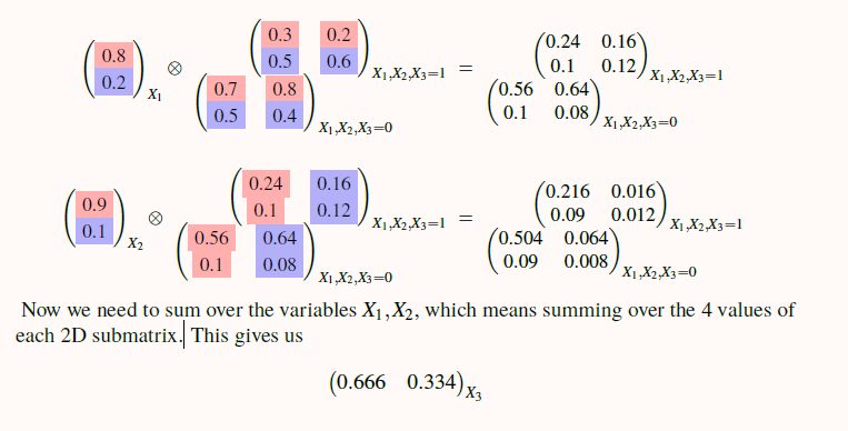
When summing, treat the two cases separately again, sum out X1, then sum out X2.