Bayesian Networks Cheatsheet
Terminology / Definitions
In Bayesian Networks one often talks in terms of family relations.
- We have parents and children for direct connections.
- We have descendants and ancestors
- Each node is trivially its own ancestor and descendant
A path in a BN may run against the arrow connections. This is a clear difference from a classic graph-theoretical concept of a path.
A Markov blanket is a set that d-separates a variable from all others in the DAG.
A structural equation model (SEM) is a Bayesian network in which each variable X is a linear function of its parents and a Gaussian variable $\epsilon_x$ called the residual.
Local Markov property: each node is independent of its non-descendants given its parents.
TIP: when writing down implied conditional independences, reason from the descendants; $descendant \ind parent | some non-descendant$.
Local and global parameter estimation: normally we estimate parameters locally at each node by conditioning on its parents. In some parametric models parameters can also be estimated globally and this can sometimes also be exploited to estimate latent variables.
Residual variance is the variance of any error (residual) and can be interpreted, I think?, as unexplained variance.
The ancestor rule is a graphical criterion for rewriting nodes in SEMs as linear combinations of residuals.
The trek rule is a graphical criterion for computing the Covariance between two variables in a SEM.
The backdoor criterion is a graphical criterion for finding adjustments sets for covariate adjustment.
A confounder is a common ancestor of X and Y in the graph where all arrows going out of X are deleted. (In most cases this is just a common ancestor, but since variables are ancestors of themselves this definition catches edge cases).
The back-door criterion and instrumental variables are methods aimed at identifying individual edge-associated parameters in a Bayesian network for causal effects.
Instrumental variables can be used when covariate adjustment using the backdoor criterion is not available, i.e. when confounders are unknown or unmeasured.
Consistency
Probability density P is consistent with G if P factorizes according to G.
Interpretation: If P is consistent with G, then all probabilities predicted by the fitted network will match the probabilities estimated directly from the data. In other words, the network will be well calibrated to the data.
A fully connected BN is trivially consistent, i.e. all independences implied by its factorization hold in P, because there are no implications. In general, this means that a consistent BN may not imply all independences that are actually in P, but it cannot imply more.
See conditional independence and faithfulness.
Tree / polytree
Tree: undirected graph with exactly one path between any pair of nodes.
Polytree: a directed graph whose skeleton is a tree (see below for skeleton)
Note that DAGs are not necessarily trees and that the skeleton of a DAG thus may have multiple paths between two given nodes. A polytree does not because its skeleton is a tree.
The class of polytrees is special because we can use factor graphs on these in polynomial time to find efficient factorizations and also produce an exact solution.
Types of networks
Skeleton: A skeleton of a DAG is a directed graph where all edges are replaced by undirected edges.
Ancestral: The ancestral network of variable $x_i$ is the subgraph of all ancestors of $x_i$ (recall: includes itself!). The ancestral graph is thus defined w.r.t. some subset of variables.
To acquire $G_a(Z)$, delete all variables except those that are ancestors of any variable in Z.
If we do Bayesian inference on the marginal probability of $x_i$ we only need the ancestral network of $x_i$, then factorize it and marginalize.
Moral: The moral graph is an undirected graph such that there are no "extramarital children". It is acquired as such:
- Connect all variables that have common children (not "grandchildren" i.e. any descendent) with an undirected edge.
- Replace all directed edges by undirected edges.
Graph pattern: If we make a mixed graph in which only the edges that are part of v-structures are drawn directed and the others undirected, then we have a graph pattern.
V-structures are not the same as colliders!
CPDAG: Some edges will change the v-structure when they change direction; so here we know their direction. If we fill in all these edges we get a CPDAG (completed partially directed acyclic graph).
Factorization
A probability density can be factorized according to DAG G if:
$$P(x_1, .., x_n) = \prod_i P(x_i | pa_G(x_i))$$
with $pa_G(x_i))$ being the set of all parents of $x_i$ in G.
This factorization holds for this specific graph.
Amount of parameters in a Bayesian Network
In the absence of a network, we need the whole joint probability distribution. E.g. for n binary variables, we then need $2^{n-1}$ parameters.
When we instead have a network and can factorize the joint probability distribution, we have that:
For p>=1, $p \times (m-1)$ with $p$ the combinations of parent values, $m$ the amount of child values; else m-1.
So do this for each node and sum up the results.
MAP
$$argmax_{h \in H} P(h|e)$$
which can be reduced to argmax over the joint distribution:
$$argmax_{h \in H} P(e,h)$$
Naive Bayes
Assume all evidence variables are independent.
$$P(e_1, .., e_n | h ) = \prod_i P(e_i | h)$$
So that MAP becomes
$$argmax_{h\in H} = P(h) \prod_i P(e_i | h)$$
which is proportional to $log(P(h)) + \sum_i log(P( e_i | h))$
Where $P(e_i|h)$ can be estimated by counting training data.
From SAT to BN
3-CNF: conjunctive normal form (conjunction of disjunctions) with <=3 literars per clause.
E.g.: ( X1 or X3 ) AND ( NOT(X1) OR NOT(X2) OR NOT(X3))
To show Bayesian exact inference is NP-hard, we need to formulate inference into a decision problem.
Recall, to show exact inference is NP-hard we translate a known NP-hard problem (e.g. 3-SAT) into a Bayesian Network. This means that if we would find a solution to exact inference in the Bayesian-network, we would also have found a solution to 3-SAT which is NP-hard. So exact inference must than at least be as hard as 3-SAT.
A: define the nodes
- Variable layer at the top (one node per variable)
- Then a clause layer (one node per clause)
- Then a formula layer (single node for the whole formula at the bottom)
B: Connect the nodes
- Draw edge from each variable to all clauses in which that variable appears
- Draw edge from each clause to the formula node
C: Construct probability table
- For binary logic, assign each variable p=0.5
- Give each clause node a probability table that encodes that clause (e.g. probability table of an OR function)
- The formula gets a table that encodes the AND operator.
For n variables and k clauses:
- n + k + (k-1) nodes
- 3k + 2(k-1) edges
- n + 8k + 4(k-1) probability table entries
Efficient Elimination Ordering
When using the distributive law to reorganize the factorization of a marginal probability or so, we can reduce $2^n$ additions (naive marginalization) to $n-1$ matrix-vector multiplications.
$P(x_2)P(x_3|x_2)$ can be interpreted as a 2x2 matrix with $X_2$ in the columns and $X_3$ in the rows.
Networks with efficient elimination orderings
A Markov Chain is a good example of a Bayesian network in which inference is not NP-Hard because it has an efficient elimination ordering. This is because we can find an elimination ordering such that we always only have to sum out one variable at a time.
This is because a Markov Chain is a polytree network. For polytree networks an efficient elimination ordering is guaranteed to exist.
The class of polytrees is special because we can use factor graphs on these in polynomial time, producing an exact solution.
Parent complexity
The presence of parents hinders the finding of efficient elimination orders.
For nodes with k parents, we need to eliminate k variables simultaneously. For all binary variables, one step requires a k-dimensional matrix with $2^k$ entries.
Elimination Order Generalized: Factor Graphs
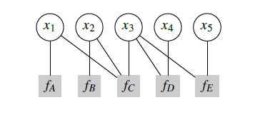
Factor graph contains:
- 1 node for each variable
- 1 node for each factor
- Edges between each factor and the variable it contains
So when "reading" the factor graph, read from the factors to the variables.
Write variables with circles, factor with squares.
See the figure for the following factorization: $f_A(x_1) f_B(x_2) f_C(x_1, x_2, x_3) f_D (x_3, x_4) f_E(x_3, x_5)$
From factor graph to expression tree of elimination ordering
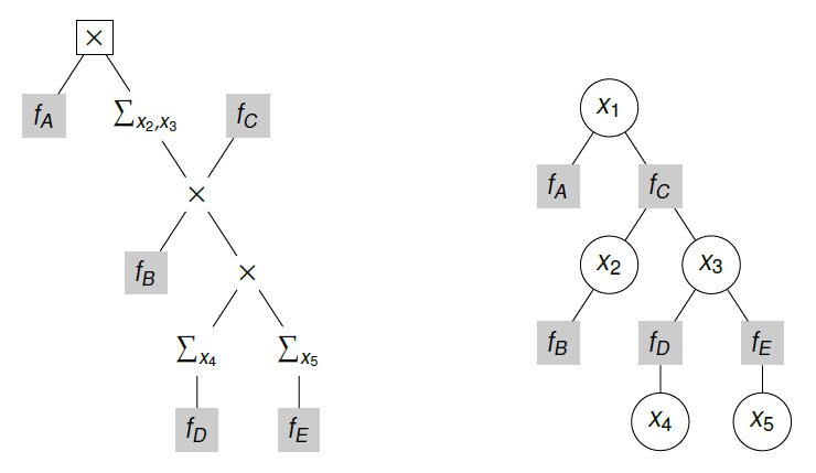
A factor graph has variable- and factor nodes.
A. Orient tree such that the desired variable becomes the tree's root node
Replacement rules:
For variable nodes:
- if x is leaf with single parent factor f, remove it
- if x is not a leaf, substitute it by the product of all its child nodes.
- N.B. the child nodes in the original graph; so before any processing
For factor nodes:
- if f is a leaf factor node with parent v, keep it as is
- else, replace with the multiplication of all children with f, then marginalize all variables except parent v, i.e. $\sum_{~{v}}$
- If there is only a single variable, you can just bypass it; this then requires further processing of the factor node later
Step by step:
- Process leaf variable nodes
- Process leaf factor nodes
- Process interior factor nodes; replace with sums except over the parent variable
- Process interior variable nodes
- When you end up with factors having other factors as children; process again with the interior factor node rule.
- When done, process root node: replaced by product of all its children
Message parsing
In practice we do not first construct an expression tree, but directly compute on the factor graph using message parsing.
The factor graph of Markov chain is still a chain. Information flow should respect parent-child relations, i.e. old orientation of edges. So to use message parsing on Markov Chains, we will orient all edges towards the root node, turning the factor graph into a tree.
Sum-Product algorithm defines a local function to each node:
- Local function at a variable node is unit function/vector (1, 1)
- Local function of factor is that factor
- Message on edge e = v -> is the product of the local function at v with all messages received on edges -> v summed over all variables except the one associated with the outgoing edge e.
The message transmitted on edge e will be a marginal distribution of the variable associated with e. So it sums up to 1. We can arbitrarily scale that to avoid numerical underflow.
This approach assumes that parents are independent! This assumption only holds for polytrees. Otherwise representing them as vectors wouldn't be enough; then we'd need covariance information as well.
For 3D, e.g. $P(X_1)xP(X_2)xP(X_3|X_1, X_2)$, separate the cases X3=0 and X3=1; notice that now the vector is a column vector and we take a regular multiplication, to clearly separate the product and sum step.
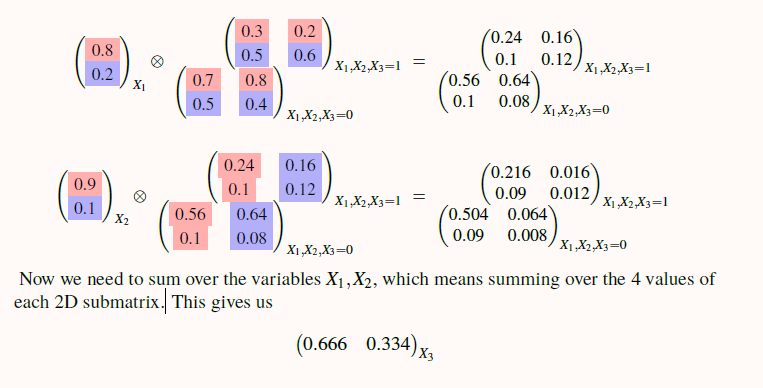
When summing, treat the two cases separately again, sum out X1, then sum out X2.
Conditional independence
- Bayesian Networks encode conditional independence assumptions
- These assumptions can be tested; false assumptions lead to incorrect inferences
- Model testing prevents wrong models, but does not prove the model is correct
Statistical Independence $X \ind Y$
$$P(x,y)=P(x)P(y)$$ $$P(x|y)=P(x)$$ $$P(y|x)=P(y)$$
Conditional independence $X \ind Y | Z$
$$P(x,y|z_1,..z_k) = P(x|z_1,...,z_k)P(y|z_1,...,z_k)$$ $$P(x|y, z_1,...,z_k) = P(x|z_1,...,z_k)$$ $$P(y|x, z_1,...,z_k) = P(y|z_1,...,z_k)$$
Shorthand notation:
$X \ind Y | A, B$ means $X \ind Y | A$ and $X \ind Y | B$.
This means that if we want to say that X and Y are conditionally independent given both A and B, we need to make explicit that it's that set: $X \ind Y | {A, B}$.
In practice, we often rely on simpler correlation measures that give an approximately correct indication of independence.
A fully connected network implies no conditional independences and is consistent with whatever data, as it cannot be falsified.
For independent variables X and Y, we still allow X -> Y in our network. This would be an error with no influence. We allow this because there is nothing in the data that falsifies this statement.
Consistency and factorizations
Probability density P is consistent with G if P factorizes according to G. So note that consistency is fully determined by conditional independences.
X -> Y factorizes as P(y|x)P(x), which holds for any P.
X Y factorizes as P(x,y)=P(x)P(y) which implies $X \ind Y$ in P.
Fork X <- M -> Y
- factorizes P(x,m,y)=P(m)P(x|m)P(y|m), implies $x \ind Y | M$
- P(x,y|m)=P(x|m)P(y|m)
Mediation X -> M -> Y implies $X \ind Y | M$
- Factorizes P(x,m,y) = P(x)P(m|x)P(y|m) = P(x|m)P(m)P(y|m)
- Then P(x,y|m)=P(x|m)P(y|m)
Collider: X -> M <- Y implies $X \ind Y$ in P.
- Factorizes P(x,m,y)=P(x)P(y)P(m|x,y)
- When we sum out m, we get P(x)P(y)
d-separation
- If X and Y are "d-separated" by Z , then ( X independent Y given Z ) is guaranteed.
- If they are not, the may or may not be conditionally independent.
So d-separation is a sufficient but not necessary criterion for conditional independence, i.e. if we have d-separation we know we have conditional independence, but non-d-separated variables may still be conditionally independent.
Smallest units of d-separation are triplets.
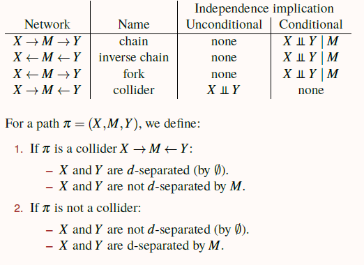
Note that only the collider has a different statistical implication, namely of marginal independence.
- A path between X1 and XN is d-separated by Z if there is a collider on the path where the middle node is not conditioned upon $X_{i-1} \rightarrow X_i \leftarrow X_{i+1}$ with $X_i \notin Z$.
- Extension: conditioning on common consequence of two variables has the same effect.
- So $X_i$ should not be an ancestor of any node in Z
- Or a non-collider (mediator in both directions, or a fork ) where the middle node is conditioned upon
Theorem Verma & Pearl, 1984:
If Z d-separates X and Y in a DAG G, then $X \in Y | Z$ in every probability density P that factorizes according to G.
d-separation in undirected graphs
A set Z d-separates X and Y in the DAG G if and only if Z separates X and Y in the ancestor moral graph $G_a(X,Y,Z)^m$.
Colliders and spurious relations
Colliders can cause spurious relations!
If you condition on the wrong thing, two unrelated variables can suddenly appear to be conditionally dependent!
Pay tuition (wealth) -> Go to uni <- Get scholarship (IQ)
Here, wealth and IQ are unrelated. But if you go to this university, you will find a negative spurious correlation between wealth and IQ. This is the consequence of conditioning on the collider; in this case only considering people that went to university.
Network testing
General problem
The basic problem with testing conditional independence between two variables X and Y given a variable Z is that X and Y could be independent given “almost all” values of Z. For example, suppose that Z is a variable that can take on a million different values, and that X and Y are only dependent given a single value ˆz. Then several million samples would be necessary to discover this dependence. Therefore, real-world tests of conditional independence need to assume that any dependence between X and Y holds for “enough” values of Z to be detected. For discrete variables, we would still be guaranteed to discover the dependence at some point, i.e., when we obtain enough samples. But for continuous variables, not even that is guaranteed. (Lecture notes, p. 122)
Categorical
Chi-square test to test independence between X and Y.
$$X^2 = \sum_{x,y} \frac{ (O_{x,y} - E_{x,y})^2 }{ E_{x,y}}$$
Chi-square compares the difference between the expected number of observations with X=x and Y=y assuming that X and Y are independent, with the actual counts of X=x and Y=y.
This means that a high chi-squared measure indicates a large deviation from the expected counts if X and Y would be independent; hence, a high chi-squared with a sufficiently low p-value) falsifies the independence assumption.
Degrees of freedom: $(n_x - 1)(n_y - 1)$ (so for binary x and y, df=1).
Requirements for valid application:
- This requires "large enough samples" (central limit theorem needs to apply)
- Smallest expected count must be large enough
- rule of thumb: at least >= 5.
Chisq for conditional independence testing.
- To test conditional independence given Z, perform the analysis on subsets of the data corresponding to values of Z, e.g. Z=0, Z=1, ... Z=k.
Problem: we end up with many p-values for individual tests.
- Combine into a single test with a single p-value
Given two tests $T_0 \sim X^2(a)$ and $T_1 \sim X^2(b)$ with a and b being degrees of freedom, then
$$T_1 + T_2 \sim X^2(a+b)$$
That is: the combined test is the sum of the statistics using the sum of the individual degrees of freedom.
Problem:
Note that chi-squared measure is very dependent on sample size. If we have many samples, we are very likely to find many very low p-values suggesting that all our assumptions are wrong. But with enough data, all variables will be somewhat related.
In addition to p-values, we therefore need to look at the effect size. One effect size is RMSEA, which takes into account chi-squared in relation to the degrees of freedom and the amount of samples.
$$RMSEA = \sqrt{ \frac{X^2 / df-1 }{N-1}}$$
- Expected RMSEA of "true" model (i.e. with the assumed independence) is 0
- Higher RMSEA means worse model fit
- For wrong model, for N->Inf RMSEA converges to positive constant; p-value converges to 0 (which is why the p-value may be misleading for large data)
N.B.
"The RMSEA is defined only for standard (unconditional) independence tests. For conditional independence tests, we can obtain RMSEA’s by computing a weighted average of the RMSEA’s of the individual chi-square tests, where each result is weighted by the number of samples that it was computed from."
Covariance and Gaussians
Var(X) = Cov(X,X) = E( (X-E(X))^2)
Cov(X,Y) = E( (X - E(X)) (Y - E(Y)))
Covariance can be seen as a measure of shared information. Note that covariance is not the same as correlation. Uncorrelated variables that do not predict each other well may still have high covariance.
Very common to use Gaussian distributions in SEMs. It is handy to have some properties ready:
For $X \sim N(\mu, \sigma^2)$ and scalar $\alpha$:
$$\alpha X \sim N(\alpha \mu, \alpha^2 \sigma^2)$$
And when adding two random normalize distributed variables:
$$X+Y \sim N(\mu_1+\mu_2, \sigma_1^2+ \sigma_2^2 + 2Cov(X,Y))$$
Example: Have X and Y both be drawn according to N(0,1) with Cov(X,Y)=0. Then Var(2X)=4 (this is a single draw). Var(X+X)=Var(X+Y)=2 (because X and Y have the same distribution we can substitute Y; X+X indicates two draws). Var(X+2Y)=5.
Linear combination property: Vector of random variables ($X_1,...,X_n$) has a multivariate normal distribution iff every linear combination of its elements has a univariate normal distribution.
Conditional covariance i.e. cov of a conditional probability distribution. This is a recursive formula:
$$Cov(X,Y|\mathbf{Z}, W) = Cov(X,Y|\mathbf{Z}) - \frac{ Cov(X,W|\mathbf{Z})Cov(Y,W|\mathbf{Z})}{ Cov(W,W|\mathbf{Z})}$$
In this special case, the specific value of Z does not matter. In the base case, just drop the conditioning on Z; these values you can read out from the covariance matrix.
SEM
A structural equation model (SEM) is a Bayesian network in which each variable X is a linear function of its parents and a Gaussian variable $\epsilon_x$ called the residual.
SEMs are usually represented as a path diagram with residual variances at the variable nodes and linear coefficients on edges. E.g. $\beta_{AZ}$ is the coefficient from A to Z.
In this course we assume for convenience the data is "centered" to mean, so we do not have to include the means in our representations.
By design, individual residuals are normally distributed; thus they have a mean estimate and we can express a standard deviation around the mean.
In standard SEMs we also assume $Cov(\epsilon_y, \epsilon_z)=0$. (We slightly change this when we have latents)
Ancestor Rule for reducing to residuals
This section is about reducing variable nodes in a SEM to a linear combination of residual terms.
Because each variable is a linear combination of its parents + Gaussian residuals, and these parents themselves are also a linear combination of its parents + Gaussian residuals, each linear combination of variables is also a linear combination of residuals.
When writing out a node only in terms of residuals, start with the parents because they are the "base case" so to say. E.g. when X has no parents, we have $X=\epsilon_X$ i.e. just the residual of variable X.
Writing out by hand is tedious. Instead, we can apply the ancestor rule.
Each variable X in SEM S can be expressed as follows:
$$X = \sum_{A \in An(X) } \sum_{paths\ p\ from\ A\ to\ X} \lambda_p \epsilon_A$$
Where $An(X) = { A | A\ is\ ancestor\ of\ X\ in\ S}$ and $\lambda_p = \prod_{U \rightarrow V\ on\ path\ p} \beta_{UV}$.
Or iteratively:
r := 0
For each ancestor A of X:
    For each path p from A to X:
        r:= r + (product of all coefficients on path p)Var(e_a)
If $p = A \rightarrow B \rightarrow C$ then $\lambda_p = \beta_{AB}\beta_{BC}$ for ancestor A and $\beta_{BC}\epsilon_B + \epsilon_c$ for ancestor B.
Remember that a node is an ancestor for itself, so we also get a $\epsilon_C$ residual from C!
Solution: $\beta_{AB}\beta_{BC}\epsilon_{A} + \beta_{BC}\epsilon_{B} + \epsilon_{C}$.
Locally fitting SEMs
You can fit nodes separately by running a linear regression of a node on its parents.
Testing conditional independence in SEMs
In multivariate Gaussian distributions, conditional independence entails a vanishing conditional covariance (=conditional covariance is 0). So if our DAG implies $A \ind C | B$ then we expect $Cov(A,C|B)=0$.
Approach 1: Compute this based on the covariance matrix (see formula above).
Approach 2: Use linear regression
$$Y = \beta_{XY}X + \beta_{ZY}Z + \epsilon_Z$$
Then $\beta_{XY} = \frac{Cov(X,Y|Z)}{Cov(X,X|Z)}$. This shows that there is a clear relation between regression coefficients and conditional covariance, meaning that we can also use the regression coefficients to test for conditional independence, because if Cov(X,Y|Z)=0 we should also find in the regression analysis that $\beta_{XY}=0$.
When testing independences, regress on the parents.
Global fitting: Implied Covariance Matrix and Trek Rule
Global estimation of parameters can be used to estimate latent variables in SEMs, using the implied covariance matrix.
Given: X -> Y -> Z, we first need to determine e.g. Cov(Y,Z). We are working towards a situation where X -> Z will have an unobserved common cause.
- Write X and Z as a linear combination of residuals
- Assume that we have mean=0, if so, then Cov(Y,Z) = E[Y*Z]
- Recall: Cov(X,Y) = E( (X - E(X)) (Y - E(Y)))
- So with means 0, E(X)=0 and E(Y)=0
- Fill in the found residual terms for Y and Z into E[Y*Z]
- Simplify
- By definition of SEM, the error terms are independent of each other, so that their covariance is 0.
- If mean=0, expectation of the product is the same as the covariance (see point 2), so we know that expectations containing a product over two different error terms will be 0, since we assumed their covariance is 0.
- This means we can keep the terms where only one error residual is involved
- Scalars i.e. path coefficients can be taken outside the expecations
$Cov(Y,Z) = \beta_{xy}^2\beta_{yz} E[\epsilon_x^2] + \beta_{yz}E[\epsilon_y^2]$ with $E[\epsilon_x^2]$ (cf. point 2) then being $Var(\epsilon_x^2)$.
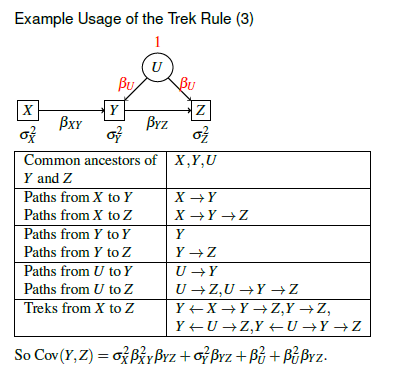
The Trek rule is a graphical criterion for determining which terms to include (and which drop out). When determining Cov(X,Y) you track down each common ancestor A and follow all possible paths down (this is a 'trek' up and down the mountain).
For each common ancestor A of X and Y:
    For each path p_x from A to X:
        For each path p_y from A to Y:
            r := r + prod. of coefficients on p_x x prod. of coeff. on p_y x Var(epsilon_A)
Latent variables
- Measurable in principle, but unmeasured
- e.g. family income may be unknown
- Conceptual variables/constructs; not measurable quantity but theoretical
- e.g. intelligence
Representation:
- Implicit: if we have two variables with a hidden common cause, we can combine their probabilities into a joint probability table.
- If they do have parents, we are forced to include the parent into that join probability table; this renders the network useless because the whole point of having a network is avoiding that table through factorizations.
- Explicit: use a parametric representation of latents
- Introduce a residual covariance $Cov(\epsilon_y, \epsilon_z)=\sigma_{YZ}^2$.
- In the case without parents we can just set it to the observed covariance between the two variables.
Approach:
- Explicitly include the latent variable U
- Assume Var(U)=1 because we can't know the unit of something we do not measure
- Set all outgoing path coefficients from U to the same value, because we have no measurement to distinguish different effect sizes anyways.
- These assumptions are necessary because otherwise the model will be unidentified for sure (i.e. we need to estimate more parameters than we have covariance entries)
N.B. having sufficient entries in the covariance matrix (i.e. >= parameters to estimate) is not a sufficient condition for the model to be identified.
Then apply the Trek Rule to find the covariance between some variables, taking into account the latent. Again, recall that a node is an ancestor of itself when determining common ancestors!
Tips:
- Write out all possible paths departing per ancestor
- For each ancestor, separate the paths to Y and the paths to Z.
- The Trek algorithm considers the combinations of paths to Y and paths to Z for each single ancestor
- Simplify: use combinations to determine 'treks' from given ancestor that visit both target variables.
- Simplify: recall that Var(U)=1 and $\beta_{UX}=\beta_{UY}=\beta_U$.
Applications with latents
-
Measurement model: we have a set of manifest variables that reflect a latent abstract concept.
- Scaling: either fix variance of latent to 1, or fix one of the path coefficients to 1
- path coefficients from latent variable to its measures are called loadings
-
Structural model: in this model we have our latents with their measures, but also causal effects between latents.
Latents in hybrid-models
Approach if all variables are either:
- Continuous
- Binary
- Ordinal
No good solution for hybrid models with categorical data.
Unbinning
Sometimes we may assume that the measure is a binning of an underlying but unmeasured continuous variable. In that case we can introduce a continuous latent variable and assume a Gaussian distribution. The binned variables occur with a particular frequency.
Thresholding:
We can then "unbin" the data by finding bounds in the Gaussian such that the cumulative density between those bounds corresponds to one of the binds.
The R-function qnorm() finds the boundary values such that the area corresponds to the frequency of the bin.
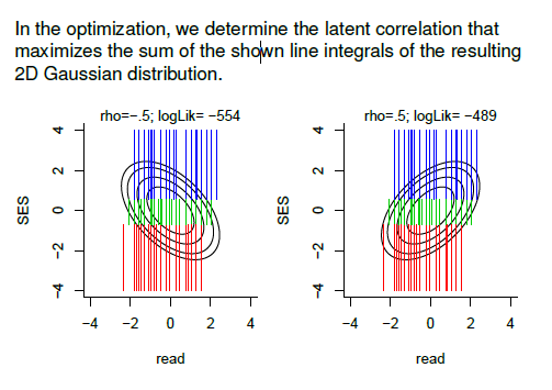
Polyserial correlation
Polyserial correlation is correlation between one continuous variable with another continuous variable that is however given in binned measurements.
Binned measure <- True measure (continuous latent) -> another continuous measure
- Infer the thresholds of the discrete latent variable (see "unbinning")
- "Optimize the value for the latent correlation to maximizes the likelihood of the data conditional on the thresholds"
Polychoric correlation
A correlation between two latent continuous variables that are both given as binned measurements.
- Infer thresholds for both discrete latent variables
- "Choose the value for the latent correlation that maximizes the likelihood of the data given the correlation and the thresholds."
Model-fitting:
- Preprocessing: if you have binned measures, represent them as ordinal data
- This is appropriate if they approximate an underlying continuous variable
- We now can estimate the polychoric correlation between any two binned ordinal measures
- This is great, because once we have this correlation, SEM fitting can be done on the correlation matrix as usual!
See Q&A recording.
Advanced conditional independence testing
Main points:
- Whenever you can compute residuals, you can test conditional independence.
- Whenever you can test conditional independence, you can quantify individual edges in a Bayesian network.
- Dummy coding and Hotelling’s test can be combined to obtain a residualization-based conditional independence test for discrete data.
We used regression for conditional independence testing.
If in a regression Y ~ X + Z the coefficient of X is 0, we conclude $Y \ind X | Z$.
But if we use linear regression in this way, this assumes our data is normally distributed ( least-squares linear regression assumes the residuals are normally distributed).
So this approach is not valid when this is not the case.
Unconditional Independence
Case: Y ~ X
Linear regression does not pick up on non-monotone relations the data, i.e. there is an increased risk of false negatives (not false positives!). FN means that our analysis suggests independence, whereas the variables are dependent. We need to find a way to use regression for non-linear data for conditional independence testing.
We can use free-form regression (e.g. local polynomial regression LOESS) or random forest to alleviate that problem.
To assess whether the regression model is appropriate, test the correlation of predictions and actual data points.
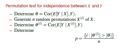
Have regression predictions $E[Y|X]$ and correlate the prediction to the actual data. If the correlation is high, then the regression is suitable for the data. We can assess the statistical significance of these correlations using a permutation test.
Permutation test
- Make a dataset where the null hypothesis is true
- So when we test for independence we make a uncorrelated dataset by randomly shuffling the data -Test correlation several times between prediction on different shuffles/permutations and data
- We then have a pretty good picture of what correlation to expect if the null hypothesis were true
- We can reject the null hypothesis if the correlation of the prediction on X with X is really different from the distribution found with the random permutations.
Modern tests like t-tests can be seen as approximating permutation tests. But in many cases we mathematically/analytically know what the null-hypothesis distribution should look like, so we don't need to "simulate" that distribution like using this permutation approach.
Permutation testing always works, no matter how complicated your data is. In well-defined cases it corresponds to the results achieved from a specific test, that is only applicable under certain circumstances.
To estimate a p-value, we can count the number of times your correlation was larger than what is expected under the null.
Conditional (in)dependence for linear relations
Case: Y ~ X + Z (where Z can be a set of variables)
Approach: test conditional independence using residuals. This is useful when the assumptions for linear regression do not hold. I.e. it is more generalizable.
- Regress X on Z and determine residuals $r_x$ = X - E(X|Z)
- Regress Y on Z and determine residuals $r_y$ = Y - E(Y|Z)
I.e. regressions are run on all other predictors Z. If $r_x$ and $r_y$ correlate, then $X \ind Y$ given Z does not hold.
rx and ry express "unique" information that's already captured by Z.
Problem: in unconditional case $Z = \O$ we can also have false positives (i.e. declare independent variables dependent).
This is because both linear regressions from above (on the residuals) may be a poor fit.
Estimate edge coefficients
See 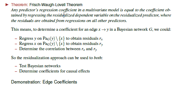
Hotelling's T^2 test for discrete data
Use dummy coding for categorical variables.
Problem: When using dummy coding, we have negative correlations between the dummy variables (they exclude each other). And the n-th dummy can be perfectly predicted by n-1 other dummies. So if we correlate some other variable with these dummy encoded columns, all these correlations will themselves be correlated.
And Hotelling's test is about checking whether a mean is 0. Mathematical trick: you can see correlation as a mean, so Hotelling's $T^2$ test is then applicable.
For conditional independence testing, each dummy variable can be residualized, e.g. by making predictions using a random forest.
The conditional independence test provides p-values. You could also use these p-values to prune edges with a very large p.
Structure learning
Consistency is fully determined by conditional independence: P is consistent with G iff every conditional independence implied by G holds in P; i.e. P factorizes according to G. So consistency means: the graph cannot be "contradicted" by the data. Note that consistency is fully determined by conditional independences.
Example: based on the data, we find $X \ind Y | M$ and nothing else. Then X M Y is not a valid solution, because when we factorize P according to G we get implied independences that were not found in the data.
Given a solution, we cannot find another solution by removing arrows because this creates new implied conditional independences. We can however add arrows, which reduces the amount of implications. The remaining implications of G will still hold in P in that case.
Consistency is too permissive for structure learning because graphs can be made trivially consistent by connecting many or all nodes. This is because then the model does not imply any conditional independences anymore and thus cannot be "contradicted" by the data.
Input: conditional independences holding in prob. distribution P
Output: a CPDAG G such that P is faithful to all DAGs represented by G (the Markov Equivalence Class of G).
Faithfulness
A BN network G is faithful to prob. distribution P when G implies exactly the set of conditional independences that hold in P. Using consistency only, it's OK to only imply a subset of the independences in P.
N.B. Faithfulness is a heuristic and we should not assume that only faithful networks are interesting; and the "true" causal diagram behind the generation of P does not need to be faithful to P.
N.B. Faithfulness is symmetric, unlike consistency.
Markov Equivalence Classes
X -> M -> Y, X <- M <- Y both imply only one conditional independence, $X \ind Y | M$
This means they are statistically equivalent, i.e. consistent with exactly the same probability distributions. Such networks are called Markov equivalent.
Graphs G and H are Markov equivalent iff:
- G and H have same skeleton
- G and H have the same v-structures
A V-structure in G is set of three variables such that U -> V <- W is an induced subgraph of G.
N.B. this implies that we do not have U -> W or U <- W; so V-structure is not the same as a collider!
V-structures imply the direction of the edges is "locked", because changing one will disrupt the V structure and change the Markov equivalence class. That is: any separating set between U and W must not include V. If we switch any edge direction, V has to be in the separating set to make U and W independent.
When you are given a graph and you should see which edges can be "undirected", then:
- Check if there are currently v-structures (!= colliders; I mess this up all the time)
- Check if switching an arrow changes that v-structure or creates a new one
Graph Patterns and CPDAGs
If we make a mixed graph in which only the edges that are part of v-structures are drawn directed and the others undirected, then we have a graph pattern.
Some edges will change the v-structure when they change direction; so here we know their direction. If we fill in all these edges we get a CPDAG (completed partially directed acyclic graph).
These are intended to be representations of equivalence classes, but they are not that easy to read. CPDAGs are suitable representations for faithful graphs.
IC algorithm (inferred causation)
Output: graph pattern that we then orient into a CPDAG.
See Q&A recording.
We can direct arrows for three reasons:
- Implied v-structures by conditional independences
- Check for arrows directions that introduce v-structures that cannot be there
-
Check for arrows that introduce cycles
-
Infer skeleton
- Start with a graph with no edges
- For each variable pair X, Y search for a set $Z_{XY}$ such that either a) $X \ind Y | Z_{XY}$ is in the input list or b)is a consequence from the implications in the input list.
- If such a set does not exist, add an undirected edge between X and Y; i.e. we have not found a possibility to make them independent, but we do not necessarily know the direction of the arrow.
- N.B. you will re-use $Z_{XY}$ for step 2
- Infer v-structure
- For each X and Y that is not linked, we check whether it has a v-structure through any neighbour W. If it has a v-structure, this would mean that W is not in separating set $Z_{XY}$, so add arrows pointing to W,
X->W<-Y. - N.B. in the other case, we leave the arrows undirected; because we have multiple equivalence classes.
- For each X and Y that is not linked, we check whether it has a v-structure through any neighbour W. If it has a v-structure, this would mean that W is not in separating set $Z_{XY}$, so add arrows pointing to W,
- Orient edges in the graph pattern where possible to create a CPDAG.
It's a simple procedure, but its complexity is terrible because it requires inspection of all subsets of variables (exponential time). So pretty unusable for any non-trivial network.
PC algorithm
Structure learning is NP-hard, but we can do better than the default IC algorithm by not starting with an empty but with a complete graph with undirected edges.
In IC we add an edge when $Z_{XY}$ does not exist. Here we take the opposite approach: when any $Z_{XY}$ exists for which $X \ind Y | Z_{XY}$, then remove the edge between X and Y. Which makes sense; otherwise they would be dependent in any case. Rest stays the same as for IC.
This is more efficient for several reasons. We can start looking for small sets $Z_{XY}$. We first start with an empty $Z_{XY}$, i.e. which variables are unconditionally independent? We can check this with a simple correlation test and using a cutoff, e.g. 0.05 correlation. This already limits the amount of subsets we have to check tremendously!
Main insight: the smaller $Z_{XY}$ the better!
Important insight: these structure learning algorithms still rely on conditional independence testing. This also means that it suffers from the same issues as we encountered before (e.g. chi-squared being unstable when conditioning upon too many things).
Interventions and Covariate Adjustment
post hoc ergo propter hoc fallacy: just because it happens afterwards does not mean it was caused by that thing.
Do-operator
Causality is investigated in an interventional rather than observational regime.
$$P(v | do(X=x)) = \prod_{X_i \in V\X} P(x_i|pa(x_i))$$
Example:
- P(cancer, coffee, smoke, U) = P(cancer | coffee,smoke) P(U) P(smoke | U) P(coffee | U)
- P(cancer, smoke, U | do(coffee)) = P(cancer | coffee,smoke) P(U) P(smoke | U)
That is, by explicitly manipulating coffee with the do operator, under controlled circumstances, we exclude possible confounding effects (U in this case).
In our Simpson Paradox example, we had a confounder that messed up our conclusion in the observational domain. Recap: if we look at the whole population the treatment was beneficial, but when selecting groups on gender not. We saw this issue was due to the trial not being randomized. Because intuitively we knew gender was a confounding factor, so intuitively we should trust the results when split on group, showing that the treatment is not effective and in fact detrimental.
We first construct prob. tables based on "seeing", i.e. in the observational regime. We have then gender as a confounder, so it may screw up our conclusions.
In the interventional regime we remove the edge between S and T (we set T) because we control who gets the treatment and who doesn't, which leads to the interventional distribution P(c,s|do(t))=P(c|s,t)P(s). We do not have any parameters of treatment t because we set it.
We can then compute (and similarly for do(T=0)):
$$P(C=1 | do(T=1)) = \sum_s P(C=1,S=s|T=1)$$ $$ = \sum_s P(C=1|S=s,T=1)P(S=s)$$
Notice that we average over sex! This is a form of covariate adjustment.
Covariate adjustment and backdoor criterion
Causal inference from observational data always requires making extra assumptions. We can encode these assumptions with BNs. Covariate adjustment formula that adjusts for confounder smoking:
$$P(cancer|do(coffee)) = \sum_{smoke}P(cancer|smoke, coffee)P(smoke)$$
Backdoor criterion: To achieve this in general settings we must find the adjustment set $Z$ for a causal effect of X on Y, such that:
- Z does not contain any descendants of X;
- Z d-separates all paths from X to Y starting with $X \leftarrow$.
- So, $X \rightarrow Y$ and $X \rightarrow M \rightarrow Y$ are fine; these are the causal effects after all
Then we have
$$P(y|do(x)) = \sum_z P(y|x,\mathbf{z})P(\mathbf{z})$$
This essentially blocks all "backdoor paths" into the cause X. One sure way of achieving this is block all parents of X.
Ex. 10.4 discusses an exception. If X is instead a set, and we include all set parents, then we can end up with a situation where the backdoor criterion fails, namely when J is a parent of X1 but a descendant of X2. The backdoor criterion excludes descendants in the adjustment set.
Backdoor criterion can be used for fitting individual causal effects.
Identifying confounders graphically
Definition of Johannes:
A confounder is a common ancestor of X and Y in the graph where all arrows going out of X are deleted.
(In most cases this is just a common ancestor, but since variables are ancestors of themselves this definition catches edge cases).
More is better case: when to condition and when not
In a regression approach, you may think "the more variables the better" because that includes its covariance; having a more precise estimate and less bias.
But Bayesian Networks show this is not simply the case. Why? Because conditioning on some variable can actually open new paths (colliders) with more noise!
E.g. ex. 10.2 is also about this. Even when a variable is not necessary to condition upon to measure an effect (i.e. it is not in the adjustment set for the causal effect of interest); it may still be worthwhile to adjust for it anyways, because e.g. in a regression analysis it would account for part of the variance. As a result, the precision of the estimate would increase.
N.B. in that case you would just include the variable in your regression model.
This can also play a role in choosing adjustment sets. Ex. 10.3 shows a choice between choosing an adjustment set with fewer variables, and one with more variables but that are all direct causes. Including direct causes can improve precision of the estimated effect.
Covariate Adjustment and Markov Equivalence
Adjustment sets are very dependent on the DAGs, but DAGs may be wrong and besides there may be many equivalent DAGs.
Johannes: can be shown however that model misspecifications are not always critical mistakes. Adjustment sets over the whole equivalence class can be very similar (meaning that you can afford a few mistakes and wrong edge orientations).
Instrumental Variables IVs
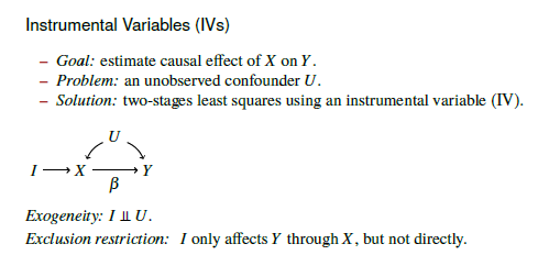
Confounding factors are often unobserved and are thus harder to account for. The backdoor criterion require us to measure and include variables of the adjustment set. But this is often not possible in practice: we often do not know the source of confounding. This is called residual confounding.
Instrumental Variables are an approach to deal with this issue, and there is a graphical criterion to identify them in BNs.
IV has two strict requirements:
- Exogeneity: I unrelated to any confounders U
- Exclusion: I only affects Y through X, but not directly
Approach two-stages least squares:
- Regress X on I and obtain prediction $X_{hat}$
- Keeps the "part of X" predict by I
- Regress Y on $X_{hat}$
X is a combination of I and U. The confounding comes from I -> X <- U -> Y. By predicting X from I only, we remove the information from U about X. We only leave the part of X that can be explained by I. We construct independence this way.
Of course $X_{hat}$ will be a noisy version of X. So the cost of this constructed independence is a loss of precision, widening the confidence interval on our prediction.
Conditional instrumental variables
Finding real instrumental variables is very hard. Finding conditional instrumental variables is a bitter better but still hard.
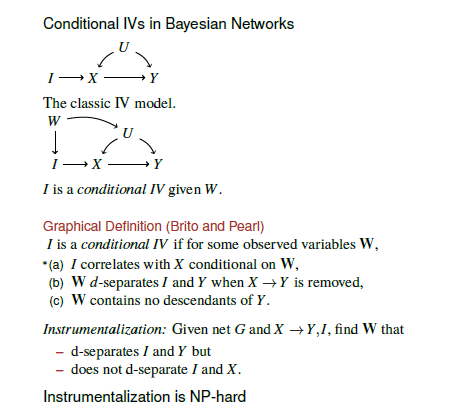
This is NP-hard, but also mainly because of some weird edge cases where conditioning on W can also introduce confounding...
Ancestral Conditional IVs
A restricted definition avoids those edge cases. The algorithm is not so important for us.
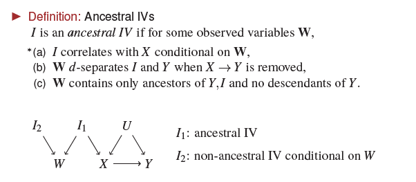 These ancestral IVs can be found more efficiently, and when we find one it's also a regular conditional IV is I understood correctly.
So it suffices to look at Ancestral IVs.