SPML Search Block
Literature:
- Poole & MacWorth 3.6.1 / 3.7-3.7.4 / 3.7.6
- Russel & Norvig: 3.5-3.5.3 / 3.6.4
Recap
- Informed search: used info about the problem to determine which node to expand next.
-
Heuristic search: sub-category of informed search where the evaluation function f is an estimate, i.e. it contains a heuristic function h that is preferably easier/faster to compute than the actual cost. E.g. A*: f(n) = g(n) + h(n)
-
Greedy algorithm: make locally best choice.
- Greedy Best-First Search (also: Greedy BFS, where the B thus does not stand for "breadth"): f(n)=h(n)
-
Downsides: stuck in local-minima (graph-search),endless cycle in local near-minima (tree-search), no optimal path guaranteed.
-
A*: f(n) = g(n) + h(n)
A*: admissibility and consistency
Optimal for Tree-search A* if heuristic h is admissible (h never overestimates).
Optimal for Graph-search A* if heuristic h is consistent, where consistency is defined as satisfying the "triangle inequality":
h(n) $\leq$ h(n') + cost(n,n') for all n, n'
If the consistency condition is met, the value of f(n) = g(n) + h(n) is monotonically non-decreasing for any partial solution on the best path to the goal.
Rationale of consistency:
At every step, if the heuristic h(n) does not overestimate the true cost of that step, the cost of step step will thus be equal or larger than its estimated cost. In other words, when this condition is met, f(n) can only stay the same or increase by making a single step.
This is a stronger condition than admissibility, which merely requires h(n) $\leq$ g(n). Therefore consistency implies admissibility but not the other way around.
A* extensions - IDA*
Complexity
IDA* improves the space complexity of A* $( O(b^m)$, exponential in path length) to O(m), linear in path length. IDA* only keeps at most 1 path in memory (like DFS).
The memory required is the number of nodes on the path to the "lowest" goal-node, which might be relatively long in terms of nodes but low in terms of costs. IDA* might also overshoot the goal, because it keeps expanding until there are no more nodes smaller than the limit value, thus required more memory than strictly speaking is necessary.
There is a small increase in time complexity though: $(b/(b-1))^2$
Algorithm description
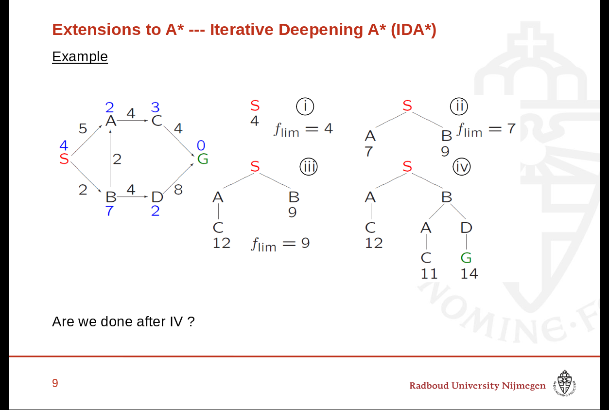
- Similar to Iterative Deepening Depth-First-Search, but expansion per iteration is sorted by increasing f-value.
- The stopping criterion is not depth, but an f-value $f_{lim}$
- Initial $f_{lim}$ = f(start-node)=h(start-node) (since g(n)=0 initially).
- For each next iteration, $f_{lim}$ is increased to the lowest f(node) $\leq f_{lim}$ in the open list (i.e. the nodes just expanded from the parent node). (This step thus also determines the stopping condition! The stopping condition is not finding a goal state, but having no more options for which f(node) $\leq f_{lim}$!
- This new $f_{lim}$ is then used for the next expansion. Expand everything until $f_{lim}$ is reached. Important: this means that expansion is not limited by depth! We can expand two nodes after each other, i.e. make two or more "steps" after each other, as long as the $f_{lim}$ is not reached.

A* Extensions - SMA*
IDA* already improves the space complexity of A, but SMA does so even further: Simplified Memory-bounded A*.
In particular, because IDA* may overshoot the goal, we cannot know exactly in advance how much memory IDA* needs. If we do exactly know how much memory we have or need, we can use SMA*.
Risk: if there is not enough memory for storing the lowest goal-node, SMA* might find an suboptimal path or be incomplete (not find the goal at all even though it exists). Also, the cheapest solution might be a longer solution.
Algorithm description:
- Updating procedure
- For (partially) unexpanded nodes: normal A* with f(n)=g(n)+h(n)
- For fully expanded nodes, f(n)=lowest f value of any descendant
- N.B. This can also be a "forgotten" value!
-
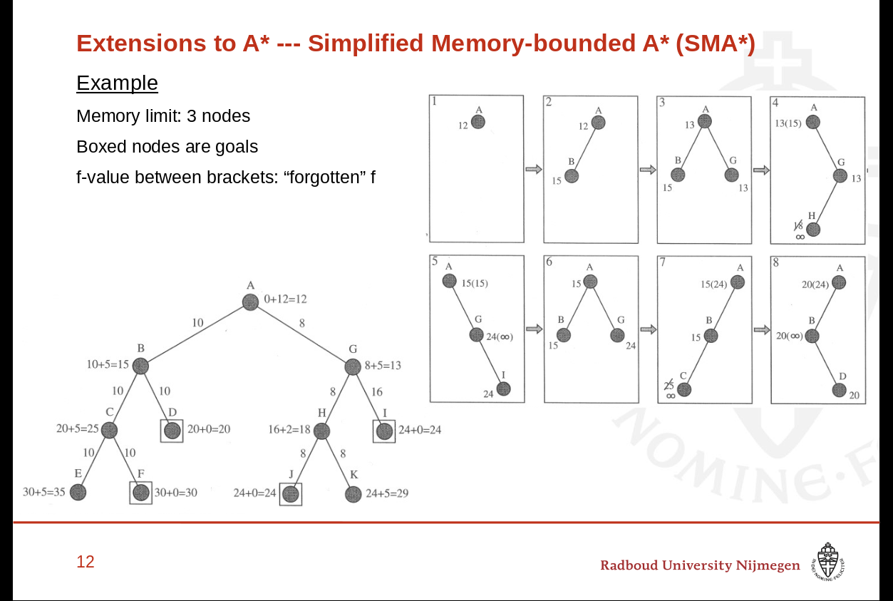
If memory limit is exceeded for a no-goal node: f(n)=$\infty$. See the example: if the memory limit is 3 and a node is the third node but not a goal, set to infinity. None of its children can ever be expanded due to the memory limit, and it is not a goal, so the node should not be visited again.
-
Forgetting
- Lowest f-value of any forgotten descendent is stored
- If memory limit reached, drop node with highest f-value from frontier. As said, the lowest f-value of forgotten children is stored at the parent node.
- The forgotten child is re-expanded if all current $f(n) > "forgotten" f(n)$
Run-through of example.
1) First step is arbitrary expansion. 2) All children of B have f values higher than 15, and G has 13, so go to G 3) Update A with the new lowest f-value: 13 4) Forget node with highest value: B. 5) Update parent A with forgotten value of B: 15. 4) H still has the lowest f-value (H18 vs I24) 5) H is not a goal node and memory limit is reached, assign infinity to it. 6) Forget node with highest f-value: which is H with infinity. 7) Update parent G with forgotten value infinity. 10) Expand I with value 24. Goal node with f=25! 11) But we do not terminate, since there still is a lower f-value: the forgotten value of B stored at A of 15. 12) Memory limit reached, so forget goal I and store it's value at parent G for possible later re-expansion. 13) Tricky! A is updated with it's lowest f-value, which is currently the forgotten value 15! 10) Now the forgotten value at A is lowest: 15 from the forgotten B. So re-expand B. 11) Forget highest f-value, which is G. NOTE: G is not set to infinity because it contains the path to the found goal! We want to retain the option to re-expand later. 12) Expand B. 13) Memory limit reached, but C is not a goal node. Set to infinity and store forgotten value at parent B. 14) Now D is has the lowest f-value. D is a goal! 15) D has f-value 20 and is a goal. There is no node with a lower f-value left (including the "forgotten" value of the previously found goal, which has f=24). So terminate.
MST's
Useful for finding the cheapest way to connect N vertices, given possible weighted and undirected connections between them.
Minimal Spanning Trees for a weighted undirected connected graph G is:
1) acyclic subgraph of G (a tree) 2) connecting all vertices (Spanning) 3) with the lowest possible sum of edge weights (Minimal)
1+3 implies that an MST always has V-1 edges (for V vertices in G)
There may be several MST's for the same graph G in case of two edges with similar weights. Consequently, there is one unique MST if all edge weights are different.
Prim's Algorithm
General idea: begin with a single root node and add one node at a time until a all vertices are connected.
Pseudo code
1) Initialize all key values with $\infty$ 3) Consider the vertices adjacent to this vertex that have not been visited yet. 4) For all adjacent vertices, update their keyvalue with the edge weight to them if it is lower than their current key value. 5) Repeat 2) Select the closest Vertex i.e. with the lowest key-value
Kruske's algorithm
General idea: start with single node trees (one for each vertex in G) and merge them by a safe edge. The subtrees in the process are themselves smaller disjoint MST's, forming a forest.
All vertices are saved in a datastructure of disjoint sets. The set A is the set containing all edges.
We require basic operations on these sets for merging into the final tree.
1) Make-set(x): add a single element x to the disjoint set 2) Find-set(x): return the key of the set containing x (and this can only be one set, because we are working with disjoint sets. 3) Union(x,y): merge the sets containing x and y respectively and destroy the original set (the latter is required to maintain disjoint sets).
Pseudocode
1) Start with an empty set of edges 2) Sort edges in nondecreasing order by weight 3) Loop over the edges (u,v) in order 4) If Find-set(u) $\neq$ Find-set(v) (i.e. they are not in the same set), then ... 5) Add the edge to the set of forest edges A but only if it connects two subtrees. 6) and merge the sets containing u and v (Union(u,v) )
Local Search - Simulated Annealing
Literature:
Poole & MacWorth: 4.8-4.8.3 Russel & Norvig: 4.1-4.1.3
Optimization Problems
An optimization problem is a problem where we do not aim to find an (optimal) path to a goal, but only an optimal solution. The paths may be absent, trivial or irrelevant.
A possible tactic using local search is to start with a non-optimal (possibly random) solution, and from there trying to find a good set of state variables that approximate a good solution.
Local search
When solutions may be anywhere, using local search to avoid looking through the whole search space for a solution, is a viable tactic. Start with an initial valuation of state variables, and try to improve on them to find the solution structure.
Local search is incomplete: not guaranteed to find and adequate or optimal solution in finite time, if there is a solution.
Some terminology:
(Random) Restart: Changing the entire set of values.
(Random) Walk: Change one (or a few) values at a time.
Random walks and/or restarts are very inefficient, and are not likely to quickly find adequate solutions unless they are really dense, i.e. a lot of possible solutions are adequate.
To improve local search we need evaluation functions for solutions, so that we can apply iterative best improvement.
Iterative Best Improvement
- Similar to greedy best-first search
- Change state to neighbour state with best evaluation (highest or lowest).
- Evaluation is usually a heuristic
- In the case of minimizing evaluation: greedy descent
- In the case of maximizing evaluation: hill-climbing
Neighbour selection using a heuristic can be divided in two stages:
1) Apply a heuristic to choose the variable to change 2) Apply a heuristic to choose the value to assign to it.
Prone to get stuck in local minima. What is a best solution for this issue depends on the solution space (or what is known of it: its evaluation/estimation).
1) A small shake (limited random walk) might be helpful for a solution space that is still quite regular. 2) In a very rough solution space (large peaks and valleys) a random restart might be needed.
Simulated Annealing
The iterative application of the idea of "shaking": start with large shakes and decrease over iterations. This amounts to moving from random search (to escape large valleys) to greedy improvement (to escape smaller subvalleys).
The basic idea is that in this method we only have walks of decreasing randomness but no restarts.
1) Random initalization of variables 2) Per iteration, randomly pick a variable to improve and pick a value for it at random 3) Decide whether to accept the newly proposed value 4) a. Always accept moves that are not a deterioration (i.e. $\geq$). b. If it is a deterioration, accept it with a probability. The worse the move, the lower the acceptance probability.
Rules for accepting a worsening move, where worsening depends on whether we want to minimize or maximize evaluation, where ... :
- h(a) is the evaluation of the original assignment, and h(a') of the new assignment.
- T is the "temperature": a value that indicates the strength of annealing. We want to start with a large amount of annealing for large T's, and slowly decrease it over time. See below: for smaller T values, the acceptance probability for worse moves decreases.
For minimizing evaluation:
p(accept)= $e^{\dfrac{h(a)-h(a')}{T}}$
Logic:
If the value we are improving is relatively large, we are more eager to accept moves (large randomness allowed). For larger T, the power $x$ approaches 0 and $e^x$ thus approaches 1. Conversely, if the value we are improving is already relatively small, we allow less randomness and thus are less likely to accept worsening moves (we only want to potentially escape small local valleys). For smaller T, the negative power $x$ is relatively large, and $e^x$ is closer to zero. See below for why the power has to be negative.
Consider the proposed move h(a'). We are only considering the acceptance probability of worsening moves (better moves are always accepted). We want to accept less worsening moves with a higher probability than moves that are way worse. In other words, if the difference between the proposed value h(a') and h(a) is relatively small, we want a higher acceptance probability. For a larger acceptance p, we need the power $x$ in $e^x$ to become smaller.
We want to minimize evaluation here. A bad move is thus when h(a') becomes bigger than h(a). When it is way bigger (a very bad move) h(a) - h(a') becomes more negative. For larger negative exponents, $e^x$ approaches zero. For a move that is only a little worse, h(a) - h(a') will still become negative but close to zero. The acceptance probability is thus closer to $e^0 = 1$.
If h(a') is really bad, and T is very low, the acceptance p approaches $e^{-\infty} = 0$
For maximizing evaluation, just turn h(a) and h(a') around:
p(accept)= $e^{\dfrac{h(a')-h(a)}{T}}$
Rule of thumb for remembering whether we want h(a)-h(a') or the other way around: for very bad moves we want the exponent to become negative, so the e power approaches zero.
So in the case of maximizing evaluation, a bad move is when h(a') is smaller than h(a). Then we can only get a negative exponent by calculating h('a) - h(a).
Annealing schedule
We still need to specify how T decreases, to force the annealing to allow less and less randomness. One possible schedule is geometric cooling. Start with T=10 and multiply with 0.97 per iteration.
Maximum Flow Networks
Literature: no required reading.
Some problems concern the flow of elements between states. The optimization of outputs given some input is a matter of finding the maximum flow.
Problem representation components:
- Unique source
- Unique sink
-
Edges with a value x/y where x denotes the actual flow and y the capacity. (So not a division).
-
Conditions are that capacities and flows are non-negative. Edges with 0/0 denote non-existing connections.
- There are no loops / edges (u,u).
- There are also no reverse connections: if (u,v) exists (v,u) is disallowed. This if for technical reasons: when this condition is met the flow network can be converted to a residual network, where for each edge a new reverse edge is introduced (which is not possible if it is already there).
These constraints are formal and workarounds are allowed:
- Given edge (u,v), (v,u) is disallowed but (v,x) with (x,u) is not.
- If a problem requires multiple sources and sinks, you can introduce a super source or super sink that connects to all other sources or sinks respectively by edges with infinite capacity (i.e. the extra edges do not change the problem at hand).
Definitions:
1) Total network flow: The sum of all f(u,v). (Easy to confuse with 4!?) 2) Capacity constraint: 0 $\leq$ f(u,v) $\leq$ c(u,v) for all edges (u,v), i.e. flows must be non-negative but cannot be larger than the capacity. 3) Flow conservation: for all vertices that are neither a source nor a sink, the sum of all input flow must equal the sum of all output flow, i.e. in intermediate vertices there can be no accumulation nor production of flow. 4) The amount of the total network flow |f| is the sum of flows f(s,u) out of source s, or the sum of flows f(u,t) into sink t. These are equivalent due to the flow conservation requirement.
Ford-Fulkerson method
A method (not an algorithm) for finding the maximum flow.
Note a method is required because one cannot simply find the maximum flow by having max capacity at all vertices, because this is very likely to violate the constraint of flow conservation, e.g. u --> (9/9) --> v --> (6/6) --> w Of course some edges also work against the current of the total flow, effectively limiting the total flow. Unnecessary extra flow might in realistic scenarios also be expensive.
Pseudo code
1) Start with zero flows for all edges. 2) Iteratively increase |f| by an augmenting path in residual network $G_f$. 3) Stop if $G_f$ does not contain any augmenting paths.
The correctness of this result is shown by the max-flow min-cut theorem.
Residual network
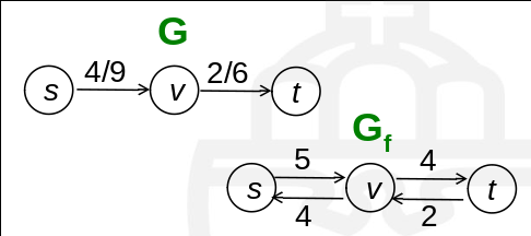
To convert a flow network to a residual network, the meaning of edges change. Whereas in a flow network an edge (u,v) indicates the flow from u to v, in a residual network the edge (u,v) means the residue i.e. potential increase in flow from u to v. In other words, capacity - current flow. Conversely, the flow at edge (u,v) is now denoted by the reverse edge (v,u). The current flow is reinterpreted as the potential decrease in flow. See the figure.
Augmenting path
An augmenting path is simply defined as a simple path in the residual network $G_f$ from source s to sink t. Can be found with a simple DFS from s to t in $G_t$.
The residual capacity is the maximum amount with which the flow on each edge of an augmenting path from s to t can be increased. In other words, since an edge now indicates the potential increase, we want to find the minimum $c_f$ over all edges (u,v) in p (i.e. if the potential increase is as low as can be, we have reached the maximum flow, considering the flow of other edges on the augmenting path).
In which situations can we improve the total network flow |f|?
a) We can increase the flow f(u,v) by the residual flow $c_f(p)$ of the whole path, if u,v is an edge in G. b) We can decrease f(v,u) by $c_f(p)$ if v,u is an edge in G (complicated way of saying that we can decrease with the maximum allowed decrease of an augmentend path p).
Basic Algorithm
1) Perform DFS to find all augmenting paths 2) While there is still an augmenting path in $G_f$, then ... 3) The residual of a path is the lowest of potential increases of every edge (u,v,) on path p. (Otherwise we exceed the capacity of one of the edges of p) 4) If (u,v) is in the original graph G, increase the flow with the potential increase of path p ($c_f(p)$) 5) If (v,u) is in the original graph G, decrease the flow with the allowed decrease of path p
Max-flow min-cut theorem
This theorem states the following equivalence:
$f is the maximum flow in G \leftrightarrow the residual network contains no augmenting paths anymore \leftrightarrow |f| = c(S,T) of a minimum cut(S,T) of G$
For the outline of the proof we need to have some definitions:
Definitions
- Cut: partition of vertices with source s on one side and sink on the other.
- Net flow f(S,T) across cut (S,T) is the summed flow all edges directly traversing the cut minus the summed flow on return edges.
- The capacity c(S,T) of a cut (S,T) is the maximum flow, i.e. the summed capacities of all edges across the cut. (No return edges considered!).
- A minimum cut has the minimum capacity of all possible cuts (S,T).
Proof outline
1) The net flow across any cut (S,T) is f(S,T) = |f|. This is self-evident: all flow from S to T must pass the cut, and what arrives at T is the inflow minus the return flow, i.e. the netto flow. 2) |f| $\leq$ the capacity c(S,T) of any cut, and thus in particular of a minimum cut. 3) To proof: |f|max = c(S,T) of a minimum cut. 4) ... we actually don't care about the proof.