Calculating pi with Monte Carlo simulation

I came across Monte Carlo sampling in a class on Bayesian statistics, where a Markov Chain Monte Carlo (MCMC) sampler was used to approximate probability distributions that were otherwise hard to calculate due to nasty integrals. This posts illustrates the basic idea of Monte Carlo sampling, by using it to approximate the number $\pi$.

The basic procedure is as follows:

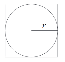
• Take a circle with radius $r$
• The area of the circle is $\pi r^2$
• Draw a containing square which then has area $(2r)^2=4r^2$.
• Sample points randomly within the square, and count how many fall within the circle
• Calculate the proportion of samples within the circle to the total amount of samples, and multiply by 4 to approximate $\pi$.

How does it work? ¶

Now we ask: what is the probability that any randomly sampled point within the square lands in the circle? This probability is the proportion of the area of the circle with respect to the total area (i.e. that of the square). We don’t want the sampling itself to influence the results, so having a uniform distribution to sample from is important.

Thus the probability that a randomly generated point lands in the circle is: $$\frac{\pi r^2}{4r^2} = \frac{\pi}{4}$$

This means that if we accurately approach the probability of a random point landing in the circle, we end up with a fourth of $\pi$. The law of large numbers states that if we repeat this experiment often enough the average of the results approaches the expected value, which is a fourth of $\pi$ in this case. It is no wonder that this method is called Monte Carlo: you might win a few games, but on average the casino always wins in the long run.

We can generate points with x and y coordinates uniformly sampled between -1 and 1. This effectively amounts to saying that for the circle we use a radius of 1, centered in (0,0). Now we need to determine a test for whether any given point lies in the circle. Given a sampled point, we can reconstruct if it lies on a circle with a radius smaller than 1. The radius is obtained with the “hypot” function, i.e. $\sqrt{x^2+y^2}$. If the reconstructed radius is smaller than the radius of our circle, we know it must lie within the circle we defined with radius 1. Otherwise, we know it is a point that only lies within the containing square, but not in the circle.

To get the probability we are interested in, we only have to divide the number of sampled points within the square by the total amount of samples. To get an approximation of $\pi$, we multiply this probability with 4.

Python script ¶

This is the python 3 script I wrote, so you can play around with the parameters yourself. The code for a simple histogram plot is also included, but you should delete this if you don’t have the matplotlib package (and don’t want to install it).

import random
import math
import matplotlib.pyplot as plt

radius=1
samples=10**6
iterations=100
countdown=iterations+1
estimations=[]

for i in range(iterations):
    sample_inside=0
    for sample in range(1,samples+1):
        hyp_r = math.hypot(random.uniform(-radius,radius),random.uniform(-radius,radius))
        if hyp_r < radius: sample_inside +=1
    countdown-=1
    print(countdown)
    estimations.append(4.0 * sample_inside / sample) 
print("Approximation of pi: ", sum(estimations)/float(iterations))
 
bins=int(iterations/2)
plt.hist(estimations, bins=bins,histtype='step')
plt.savefig("pi-plot.png")

Sampling and Plots ¶

Another question is how much samples we need: a lot. Without working out the mathematics, some quick and dirty testing shows that in order to get only one decimal accuracy we already need at least 10.000 samples. Unfortunately, to get more accuracy, we need relatively more and more samples, since the rate of convergence is the inverse of the square root of the number of samples N. In simple words: the higher the number of samples we take, the slower the convergence.

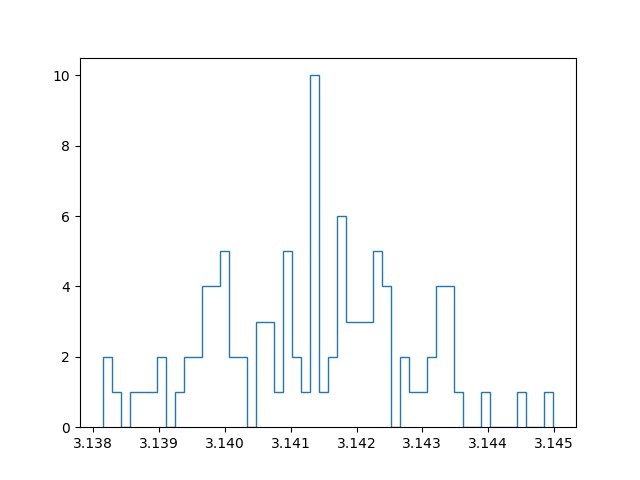
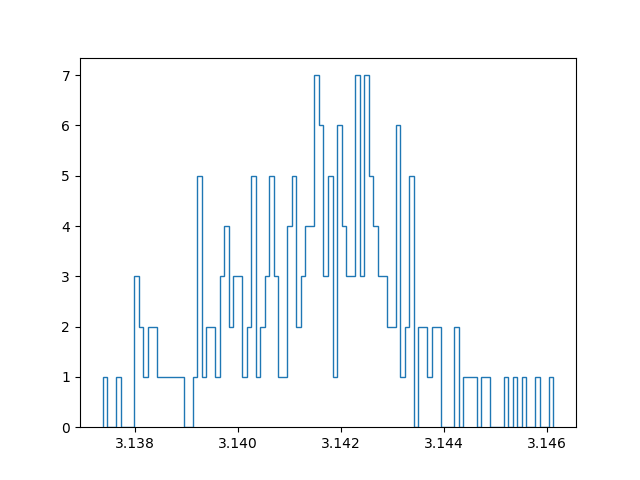
With a million samples, we can approximate the first two decimals well, but for the third decimals we already start getting into trouble. On top of that, the approximation becomes slow… Instead of straightforwardly pumping up the number of samples taken to increase the accuracy, I tried out another strategy. Instead of running a simulation with for example 100 million samples, I tried running 100 simulations with a million samples, and taking the average of those for the final approximation. In this manner we can create a confidence interval and say something about how reliable our estimate is. Since all samples are independent and concern a stochastic variable, the central limit theorem applies. In other words: if we have enough approximations, these approximations themselves will follow a normal distribution. I have an ongoing discussion with some friends about the benefit of this method, compared to running one bigger simulation. My current position is that with taking the mean over multiple approximations (which are themselves means over a million samples), we have a lower maximum precision than a single run with the same amount of total samples, but effectively get a better estimate because the result is more reliable.

Below are plots using a million samples and 100 and 200 iterations respectively. We indeed see that the means of the iterations crudely follow a normal distribution.